In my article on computing confidence intervals for rankings, I had to generate p random vectors that each contained N random numbers. Each vector was generated from normal distribution with different parameters. This post compares two different ways to generate p vectors that are sampled from independent normal distributions.
Sampling from Normal Distributions in SAS/IML
Recall that the following SAS/IML statements sample from p identical normal distributions:
proc iml; call randseed(1234); /** set random number seed **/ N = 10000; /** number of observations per sample **/ p = 100; /** number of variables **/ mean = 1; stdDev = 2; x = j(N, p); /** allocate space for results **/ call randgen(x, "Normal", mean, stdDev); |
Each of the p columns of the matrix x is a sample from the same normal population. Today's article describes how to sample each column from a different population. That is, the means and standard deviations are different for each column of x.
As I've discussed previously, when you want correlated vectors you can sample from a multivariate normal distribution by using the RANDNORMAL module. Each of the resulting vectors is univariate normal and they are correlated with each other.
You can also use the RANDNORMAL module to sample from p independent and uncorrelated variables: just pass in a diagonal matrix for the covariance matrix. However, there is a more efficient way to sample from p independent normal variables: call the RANDGEN function p times in a loop.
Why Sampling in a Loop Is Better
Some long-time readers might be surprised that I would recommend writing a loop because I have blogged many times about the evils of unnecessary looping in the SAS/IML language, especially for sampling and simulation. But loops are not inherently evil. The point I often make is that loops should be avoided when there is a more efficient vectorized function that does the same thing.
But in the case of sampling from independent normals, a loop is more efficient than calling the RANDNORMAL module. Here's why. The RANDNORMAL algorithm has three steps:
- Sample from p independent standard normal distributions.
- Compute the Cholesky decomposition of the covariance matrix by using the SAS/IML ROOT function.
- Perform a matrix multiplication that transforms the uncorrelated variates into correlated variates.
Because the RANDNORMAL algorithm requires sampling, but also involves a Cholesky decomposition (which is an O(p3) operation), I expect it to be less efficient than an operation that uses only sampling.
The following statements use PROC IML to compute p independent normal variates, each with its own mean and variance:
mean = j(p,1,0); /** use zero means **/ var = uniform( j(p,1) ); /** random variances **/ x = j(N, p); /** allocate space for results **/ z = j(N,1); /** allocate helper vector **/ do i = 1 to p; call randgen(z, "Normal", mean[i], sqrt(var[i])); x[,i] = z; end; |
Comparing the Two Algorithms
For comparison, the following statements sample from a multivariate normal distribution with uncorrelated components:
D = diag(var); /** diagonal covariance matrix **/ x = randnormal(N, mean, D); |
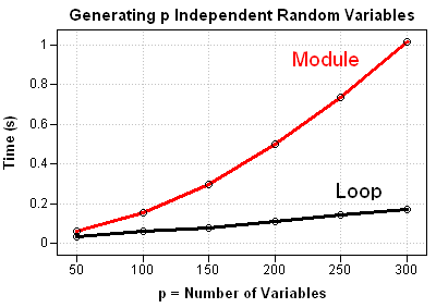
You can use the techniques in Chapter 15 of my book, Statistical Programming with SAS/IML Software, to compare the performance of these two methods for a range of values of p. A graph of the results shows that the RANDNORMAL method does indeed require more computational time. Using the module, it takes about one second to create a 300x300 covariance matrix and use it to generate 300 random vectors with 10,000 observations. If you use a loop, sampling from 300 univariate normal distributions takes less than 0.2 seconds.
So go ahead and loop. This time, it's the more efficient choice.


3 Comments
Pingback: Generate a random sample from a mixture distribution - The DO Loop
In SAS9.4 , it supported vector MEAN and STD. It is amazing .
proc iml;
mu={0 2 4};
sigma={3 4.5 16};
x=j(10000,3);
call randgen(x,'normal',mu,sigma);
mean=mean(x);
std=std(x);
print mean,std;
quit;
The MEAN and STD functions were introduced way back in SAS 9.22. See this article.