In a previous article, I showed two ways to define a log-likelihood function in SAS. This article shows two ways to compute maximum likelihood estimates (MLEs) in SAS: the nonlinear optimization subroutines in SAS/IML and the NLMIXED procedure in SAS/STAT. To illustrate these methods, I will use the same data sets from my previous post. One data set contains binomial data, the other contains data that are lognormally distributed. You can download the SAS program that creates the data and computes these maximum likelihood estimates.
Maximum likelihood estimates for binomial data from SAS/IML
I previously wrote a step-by-step description of how to compute maximum likelihood estimates in SAS/IML. SAS/IML contains many algorithms for nonlinear optimization, including the NLPNRA subroutine, which implements the Newton-Raphson method.
In my previous article I used the LOGPDF function to define the log-likelihood function for the binomial data. The following statements define bounds for the parameter (0 < p < 1) and provides an initial guess of p0=0.5:
/* Before running program, create Binomial and LN data sets from previous post */ /* Example 1: MLE for binomial data */ /* Method 1: Use SAS/IML optimization routines */ proc iml; /* log-likelihood function for binomial data */ start Binom_LL(p) global(x, NTrials); LL = sum( logpdf("Binomial", x, p, NTrials) ); return( LL ); finish; NTrials = 10; /* number of trials (fixed) */ use Binomial; read all var "x"; close; /* set constraint matrix, options, and initial guess for optimization */ con = { 0, /* lower bounds: 0 < p */ 1}; /* upper bounds: p < 1 */ opt = {1, /* find maximum of function */ 2}; /* print some output */ p0 = 0.5; /* initial guess for solution */ call nlpnra(rc, p_MLE, "Binom_LL", p0, opt, con); print p_MLE; |
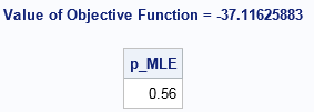
The NLPNRA subroutine computes that the maximum of the log-likelihood function occurs for p=0.56, which agrees with the graph in the previous article. We conclude that the parameter p=0.56 (with NTrials=10) is "most likely" to be the binomial distribution parameter that generated the data.
Maximum likelihood estimates for binomial data from PROC NLMIXED
If you've never used PROC NLMIXED before, you might wonder why I am using that procedure, since this problem is not a mixed modeling regression. However, you can use the NLMIXED procedure for general maximum likelihood estimation. In fact, I sometimes joke that SAS could have named the procedure "PROC MLE" because it is so useful for solving maximum likelihood problems.
PROC NLMIXED has built-in support for computing maximum likelihood estimates of data that follow the Bernoulli (binary), binomial, Poisson, negative binomial, normal, and gamma distributions. (You can also use PROC GENMOD to fit these distributions; I have shown an example of fitting Poisson data.)
The syntax for PROC NLMIXED is very simple for the Binomial data. On the MODEL statement, you declare that you want to model the X variable as Binom(p) where NTrials=10, and you use the PARMS statement to supply an initial guess for the parameter p. Be sure to ALWAYS check the documentation for the correct syntax for a binomial distribution. Some functions like PDF, CDF, and RAND use the p parameter as the first argument: Binom(p, NTrials). Some procedure (like the MCMC and NLMIXED) use the p parameter as the second argument: Binom(NTrials, p).
/* Method 2: Use PROC NLMIXED solve using built-in modeling syntax */ proc nlmixed data=Binomial; parms p = 0.5; * initial value for parameter; bounds 0 < p < 1; NTrials = 10; model x ~ binomial(NTrials, p); run; |
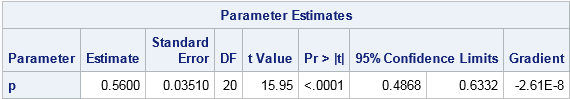
Notice that the output from PROC NLMIXED contains the parameter estimate, standard error, and 95% confidence intervals. The parameter estimate is the same value (0.56) as was found by the NLPNRA routine in SAS/IML. The confidence interval confirms what we previously saw in the graph of the log-likelihood function: the function is somewhat flat near the optimum, so a 95% confidence interval is wide: [0.49, 0.63].
By the way, both PROC IML and PROC NLMIXED enable you to choose your favorite optimization solver. In this example, I used Newton-Raphson (CALL NLPNRA) for the SAS/IML solver, but you could also use a quasi-Newton solver (the NLPQN subroutine), which is the solver used by PROC NLMIXED. Or you can tell PROC NLMIXED to use Newton-Raphson by adding TECHNIQUE=NEWRAP to the PROC NLMIXED statement.
Maximum likelihood estimates for lognormal data
You can use similar syntax to compute MLEs for lognormal data. The SAS/IML syntax is similar to the binomial example, so it is omitted. To view it, download the complete SAS program that computes these maximum likelihood estimates.
PROC NLMIXED does not support the lognormal distribution as a built-in distribution, which means that you need to explicitly write out the log-likelihood function and specify it in the GENERAL function on the MODEL statement. Whereas in SAS/IML you have to use the SUM function to sum the log-likelihood over all observations, the syntax for PROC NLMIXED is simpler. Just as the DATA step has an implicit loop over all observations, the NLMIXED procedure implicitly sums the log-likelihood over all observations. You can use the LOGPDF function, or you can explicitly write the log-density formula for each observation.
If you look up the lognormal distribution in the list of "Standard Definition" in the PROC MCMC documentation, you will see that one parameterization of the lognormal PDF in terms of the log-mean μ and log-standard-deviation σ is
f(x; μ, σ) = (1/(sqrt(2π σ x) exp(-(log(x)-μ)**2 / (2σ**2))
When you take the logarithm of this quantity, you get two terms, or three if you use the rules of logarithms to isolate quantities that do not depend on the parameters:
proc nlmixed data=LN; parms mu 1 sigma 1; * initial values of parameters; bounds 0 < sigma; * bounds on parameters; sqrt2pi = sqrt(2*constant('pi')); LL = -log(sigma) - log(sqrt2pi*x) /* this term is constant w/r/t (mu, sigma) */ - (log(x)-mu)**2 / (2*sigma**2); /* Alternative: LL = logpdf("Lognormal", x, mu, sigma); */ model x ~ general(LL); run; |
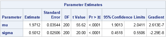
The parameter estimates are shown, along with standard errors and 95% confidence intervals. The maximum likelihood estimates for the lognormal data are (μ, σ) = (1.97, 0.50). You will get the same answer if you use the LOGPDF function (inside the comment) instead of the "manual calculation." You will also get the same estimates if you omit the term log(sqrt2pi*x) because that term does not depend on the MLE parameters.
In conclusion, you can use nonlinear optimization in the SAS/IML language to compute MLEs. This approach is especially useful when the computation is part of a larger computational program in SAS/IML. Alternatively, the NLMIXED procedure makes it easy to compute MLEs for discrete and continuous distributions. For some simple distributions, the log-likelihood functions are built into PROC NLMIXED. For others, you can specify the log likelihood yourself and find the maximum likelihood estimates by using the GENERAL function.

21 Comments
Rick, you say /* Before running program, create Binomial and LN data sets from previous post */, yet when I follow the link to the previous post all I find is the Fisher Iris data!
Sorry for the confusion. The link that contains the data came later. I added a new link earlier to make it easier to find the data. Search for the word "download" on this page.
How would you interpret a MLE for a NL transformed lognormal variable. It would be on the log normal scale, so is it interpreted as a percentage, just a log version, or can you back transform it into a log normal value?
Sorry, but I don't understand what you mean by "interpret." The parameters that optimize the ML are those which are most likely, given the data. If the "NL transformation" is monotonic, the same parameters maximize the likelihood of the r.v AND the transformed r.v. If that doesn't help, you can ask your question on a discussion forum. Since your question does not involve SAS programming, I suggest https://math.stackexchange.com
Hello!
PROC NLMIXED is very nice to compute ML estimators, but how can I "export" the parameters? Is it an option to create output dataset(s)?
Best regards
Michel.
It sounds like you want to save the ParameterEstimates table to a data set. Use
ods output ParameterEstimates=PE;
as described in the article "ODS OUTPUT: Store any statistic created by any SAS procedure."
I was able to use this code to get the parameter estimates that I would like but I need confidence intervals for the model parameters that are estimated using the likelihood profile method. Is there a way to do this using proc nlmixed? Here is the code I am using:
/*create data table that includes Q*/
PROC SQL;
CREATE TABLE WORK.SEIDMANETAL1986_Q AS
SELECT t1.TSFE_yrs_Range,
t1.TSFE_yrs_Avg,
t1.duration,
t1.conc,
t1.PY,
t1.'Obs'n,
/* Q */
(case
when t1.TSFE_yrs_Avg=. then .
when t1.TSFE_yrs_Avg(10+t1.duration) then (t1.TSFE_yrs_Avg-10)**3-(t1.TSFE_yrs_Avg-10-t1.duration)**3
else (t1.TSFE_yrs_Avg-10)**3
end) AS Q
FROM '\\Esc-server1\home\rshaw\EH027\seidmanetal1986.sas7bdat' t1;
run;
/*model*/
proc nlmixed data=WORK.SEIDMANETAL1986_Q;
parms KM 1e-08; /*starting value*/
pred = conc*KM*Q*PY;
ll=LogPDF("POISSON",Obs,Pred); /*LofPDF function Returns the logarithm of a probability density (mass) function. Poisson distribution is specified.*/
model Obs ~ general(ll);
predict pred out=model1; /*generates table with predicted values and CI’s titled “Model1”*/
run;
PROC NLMIXED computes the confidence limits for parameters by default. See the ParameterEstimates table.
Pingback: Two simple ways to construct a log-likelihood function in SAS - The DO Loop
Hi Rick, thanks for the nice knowledge. I am wondering could we draw the curve due to the parameters from the procedure? for example, we could draw the normal distribution bell curve with the histogram graph.
Yes. An example is in one of the links.
Hello Rick, I'm trying to estimate the equation 5 of this paper: https://www.scielo.br/scielo.php?script=sci_arttext&pid=S0034-71402016000400441. Do you have any reference to obtain the parameter results?. Please I'm searching more information but I don't find nothing. Thank you so much.
Sorry, but I do not have any references for you. The best I can suggest is to post your question to the SAS Support Communities.
Hello. Could you tell us a bit more about "NTrials"? I am running the proc nlmixed for lognormal data and the result is quite variable by the value of NTrials. I don't see anything about this statement online. Thanks!
NTrials is not a statement. It is the parameter to the binomial distribution, usually called "N".
Pingback: The knapsack problem: Binary integer programming in SAS/IML - The DO Loop
Hello Dr. Rick
I m developing wilmink model for cattle lactation data set.. I need to run NLMIXED in sas. this model has 4 parameters and one predictor variable.
so please help me to write the SAS codes for that.
I used following codes. but I dont know how to write them. please help me
Data Lactation;
Input Parity DIM Yield;
Cards;
8 1 .
;
proc nlmixed;
parms a=5, b=0.1, c=0.1, d=0.1;
model yield = a-(b*dim)-(c*exp(-d*dim));
random a b c d ([0,0,0,0}, ) subjects =
run;
You can get help on SAS programming by posting your question on the SAS Support Communities. For this question, I recommend the Statistical Community.
Pingback: Standard errors for maximum likelihood estimation - The DO Loop
Pingback: Maximum likelihood estimates for linear regression - The DO Loop
Pingback: Use a high-low plot to emulate a histogram in SAS - The DO Loop