I have previously shown how to overlay basic plots on box plots when all plots share a common discrete X axis. It is interesting to note that box plots can also be overlaid on a continuous (interval) axis. You often need to bin the data before you create the plot.

A typical situation when you plot a time series. You might want to overlay box plots to display a summary of the response distribution within certain time intervals. For example, last week I visualized World Bank data for the average life expectancy in more than 200 countries during the years 1960–2014. Suppose that for each decade you want to draw a box plot that summarizes the response variable for all countries. You can use the DATA step (or create a data view) to create the Decade variable, as follows:

data Decade / view=decade;
set LE;
if      1960 <= Year <= 1969 then Decade=1965;
else if 1970 <= Year <= 1979 then Decade=1975;
else if 1980 <= Year <= 1989 then Decade=1985;
else if 1990 <= Year <= 1999 then Decade=1995;
else if 2000 <= Year <= 2009 then Decade=2005;
else if 2010 <= Year         then Decade=2015;
else Decade = .;   /* handle bad data */
run;

You can use the following call to PROC SGPLOT to overlay the box plot and the scatter plot of the data:

/* overlay data by year and box plots to summarize decades */
title "Distribution of Life Expectancy by Decade";
title2 "Raw Data for 207 Countries by Year";
proc sgplot data=Decade noautolegend;
   vbox Expected / category=Decade;              /* box plot */
   scatter x=year y=Expected / transparency=0.9; /* semitransparent scatter */
   xaxis type=linear display=(nolabel)           /* linear axis */
         values=(1965 to 2015 by 10)             /* optional: set ticks labels */
         valuesdisplay=('60s' '70s' '80s' '90s' '2000s' '2010s');
run;

There are a couple of tricks that make this overlay work:

• The discrete Decade variable uses the same scale as the continuous Year variable. In fact, the Decade value is in the middle of the continuous interval for each decade.
• The scatter plot markers are highly transparent so that they show the individual measurements without overwhelming the display.
• The TYPE=LINEAR option in the XAXIS statement enables you to overlay the scatter plot which has an interval X axis) and the box plot (which has discrete X values).
• Optionally, you can specify the location of the major tick marks by using the VALUES= option in the XAXIS statement. In this example, the tick marks are set to be 1965, 1975, and so forth, which are the values of the Decade variable. To emphasize the decades, rather than particular years, you can use the VALUESDIPLAY= option to manually set the values that are displayed for each tick mark.

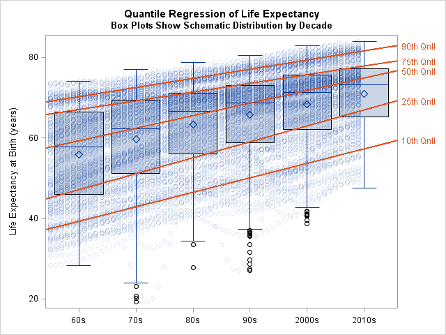
Overlay regression lines on box plots

In my previous article I showed how you can use the CONNECT= option to connect quantiles of adjacent box plots. Some people use the CONNECT= option as a poor man's version of quantile regression. However, quantile regression is more than merely connecting the sample quantiles of binned data. Quantile regression shows trends for various quantiles of the response variable.

For brevity, I will not discuss how to use PROC QUANTREG to perform quantile regression on these data. However, you can download the program that performs the analysis and creates the graph.

The graph overlays quantile regression lines on the previous graph. Notice that the 90th and 75th quantiles of life expectancy are increasing at a rate of about 2 years per decade. The median life expectancy is increasing at a faster rate of 3 years per decade. The lower quantiles are increasing even faster: the 25th quantile is increasing at about 4 years per decade and the 10th quantile is increasing at about 3.6 years per decade. Notice that the 25th, 50th, and 75th quantile curves are close to (but not equal to) the corresponding features of the aggregated box plots.

I think that this graph provides an excellent visualization of trends in life expectancy around the world, especially if combined with spaghetti plots or lasagna plots. The countries at the top of the plot have good sanitation, health care, and nutrition. Consequently, their life expectancy increases at a slower rate than countries that have poorer sanitation and nutrition. Small improvements in the poorer countries can make a big difference in the life expectancy of their population.

Summary

In summary, you can overlay continuous plots and box plots in SAS 9.4m1. You need to ensure that the categories of the box plots are on the same scale as the continuous X variable. You need to set the TYPE=LINEAR option on the XAXIS statement. Lastly, you might want to use partial transparency to ensure that the graph doesn't become too crowded.