You've probably heard of a random walk, but have you heard about the drunkard's walk? I've previously written about how to simulate a one-dimensional random walk in SAS. In the random walk, you imagine a person who takes a series of steps where the step size and direction is a random draw from the normal distribution. The drunkard's walk is similar, but the drunkard takes unit steps in a random direction (for example, left or right in one dimension).

For both kinds of walks, you can create a simulation by drawing the step at random. To find the walker's path, you form the cumulative sum of the steps.

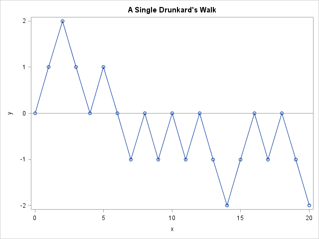
In a one-dimensional drunkard's walk, the drunkard takes a step to the left or to the right with probability 0.5. In the SAS DATA step, you can use the RAND function to draw from the Bernoulli distribution. You can do the same in the SAS/IML language, but SAS/IML also supports the SAMPLE function, which you can use to directly sample from a finite set such as {+1, -1}. The following SAS/IML statements simulate a drunkard's walk that begins at 0 and proceeds for 20 steps. A line plot of the drunkard's path is shown.

proc iml;
call randseed(1234);
NumSteps = 20;
x = sample({-1 1}, 1 // NumSteps);  /* 1 col; NumSteps rows */
position = x[+];                    /* final position of drunkard */
Y = cusum(0 // x);                  /* show initial position at t=0 */
title "A Single Drunkard's Walk";
call series(0:NumSteps, Y) other="refline 0/ axis=y;" option="markers";

For this choice of the random number seed, the drunkard's final position is two units to the left of his original position. If you change the random number seed and rerun the program, the final position might be -4 for some runs, +2 for others, and 0 for some others. However, the final position after 20 steps cannot be an odd number of units. When the drunkard takes an even number of steps, the difference between his final and initial positions is even; when he takes an odd number of steps, the difference is odd.

You can easily simulate 5,000 drunkards who all start at position 0. In the following simulation, each drunkard staggers randomly for 100 steps. The histogram shows the distribution of the positions of the 5,000 drunkards:

proc iml;
call randseed(1234);
NumWalks = 5000;
NumSteps = 100;
x = sample({-1 1}, NumWalks // NumSteps); /* 5000 columns; NumSteps rows */
position = x[+,];                     /* final position of each drunkard */
 
title "Final Position of 5,000 Drunkards";
call histogram(position) xvalues=do(-40,40,2) rebin={-38,2};

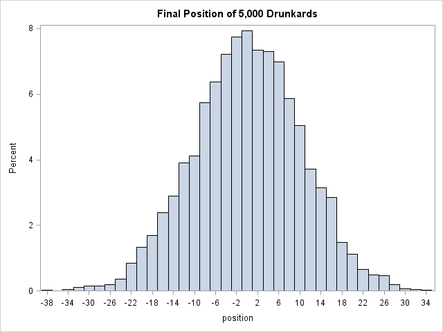
The final position is distributed like a binomial distribution, but with a twist. When n is even (as in this case), all the probability density is restricted to the even positions; when n is odd (such as the 99th step), the density is on the odd positions.

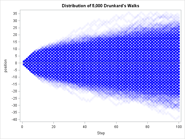
You can create a time series by forming the cumulative sums of the steps. The simulation created a matrix where each column represents the path of a single drunkard. To plot all of the paths on a single graph, it is convenient to convert the data from wide to long form. Then a call to the SCATTER routine plots all of the positions. The markers are semi-transparent so that overplotted points appear darker and the plot gives some indication of the density of the positions.

/* create time series for each drunkard */
Y = j(nrow(x), ncol(x));
do i = 1 to NumWalks;
   Y[,i] = cusum(x[,i]); /* just show steps 1..N */
end;
 
/* https://blogs.sas.com/content/iml/2015/02/27/multiple-series-iml.html */
load module=WideToLong;         /* or insert the module definition here */
run WideToLong(Position, Step, group, Y);
 
title "Distribution of 5,000 Drunkard's Walks";
call Scatter(Step, Position) group=group 
        option="transparency=0.95 markerattrs=(symbol=SquareFilled color=blue)" 
        procopt="noautolegend" yvalues=do(-40,40,5) other="refline 0 / axis=y;";

In conclusion, the drunkard's walk is an interesting variation of the random walk. In the drunkard's walk, the step size is always unit length. The location of a drunkard after n steps follows a binomial distribution on even or odd positions.

Although I demonstrated this simulation by using the SAS/IML language, it is straightforward to reproduce these results by using the DATA step and the SGPLOT procedure. I leave that exercise for the motivated reader.