Last month I wrote about how to simulate a drunkard's walk in SAS for a drunkard who can move only left or right in one direction. A reader asked whether the problem could be generalized to two dimensions. Yes! This article shows how to simulate a 2-D drunkard's walk, also called a random walk becuase each step is taken in a random direction.

In fact, it is possible to simulate the drunkard's walk in d dimensions. The drunkard starts at the origin of the coordinate system. He chooses a random coordinate direction and takes a unit step in either the positive or negative direction for that coordinate. If the drunkard takes N steps, you can determine the probability that the drunkard is in a particular location.

The computational methods used to simulate a random walk in higher dimensions are similar to the 1-D walk, so see my previous article for the background information.

Visualizing a drunkard's walk

In two dimensions, you can use a series plot to visualize the path of the drunkard as he stumbles to the north, south, east, and west. The following PROC IML program uses the Table distribution to draw 10 random values from the set {1, 2}, which are the two coordinate directions. The SAMPLE function makes random draws from the set {-1, 1} and determines whether the drunkard steps forward or backward in the chosen coordinate direction:

proc iml;
call randseed(54321);
dim = 2;                   /* number of directions */
NumSteps = 10;             /* number of steps */
 
coord = j(NumSteps,1,.);   /* allocate vector for random direction */
call randgen(coord, "Table", j(1,dim,1)/dim); /* random directions */
incr = sample({-1 1}, 1 // NumSteps);         /* random step +/-1 */
step = T(1:NumSteps);
print step coord incr;

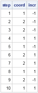
The value coord=1 means that the drunkard takes a step in the x direction. The value coord=2 means that the drunkard steps in the y direction. The table shows that the drunkard's first step is a backward step in the x direction (west). The next step is a negative step in the y direction (south), and so forth. The complete trajectory is west, south, south, east, west, north, north, east, south, and east.

These two random vectors can be combined to form an N x d matrix where each column is a coordinate direction, each row is a time step, and the values 1, -1, and 0 indicate that the drunkard moves forward, backward, or does not move, respectively. This matrix contains the same information as the previous table. You can use the SUB2NDX function to convert subscripts into indices, and therefore create the matrix, as follows:

x = j(NumSteps, dim, 0);      /* (N x d) array */
idx = sub2ndx(dimension(x), step||coord);
x[ idx ] = incr;
print x;

You can encapsulate the preceding statements into a module that implements the Drunkard's Walk algorithm. You can download the complete SAS program that generates the graphs and computations in this article.

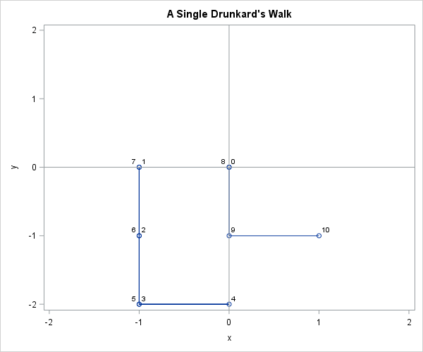
To visualize the path, you can use the CUSUM function on each column of the x matrix to accumulate the steps. The accumulation creates a new matrix that contains the position of the drunkard after each step. The following series plot attempts to show the path of the drunkard, with locations labeled by time. For most random walks, there is considerable overplotting. The graph show that the drunkard started at the origin and sequentially moved west, south, south, east, west, and so forth. The final position of the drunkard is at (1, -1). This path is typical in that the drunkard staggers near the origin. Although it is possible for the drunkard to always choose the same direction, it is not probable.

Visualizing the probability distribution of the final position

Just as in the one-dimensional case, you can use simulation to visualize the probability distribution of the final position of the drunkard. If the drunkard takes an even number of steps, he must end up an even distance away from the origin, where the distance is calculated by using the Minkowski metric, also known as the "Manhattan" or "taxicab" metric. The probability is highest that the drunkard returns to the origin, followed by the points that are two units away, four units away, and so forth. The following SAS/IML statements call the DrunkardWalk function 10,000 times and plots the counts for each final position by using a heat map:

/* Assume DrunkardWalk function is defined (see link to program).
   Compute final positions of 10,000 walks */
NumSteps = 6;
NumWalks = 10000;
finalPos = j(NumWalks, dim);
do i = 1 to NumWalks;
   x = DrunkardWalk(dim, NumSteps);
   finalPos[i,] = x[+,];
end;
 
create walk from finalPos[c={"x" "y"}];   /* write to SAS data set */
append from finalPos;
close;
submit;
   proc freq data=walk noprint;           /* PROC FREQ computes counts */
   tables x*y / list sparse out=freqOut;
   run;
endsubmit;
/* read results back into SAS/IML vectors */
use freqOut;   read all var {x y count};   close;
 
/* reshape counts into rectangular matrix and visualize with heat map */
nX = range(x) + 1;
nY = range(y) + 1;
W = shape(count, nX, nY);
call HeatmapCont(W) xValues = unique(x) yValues=unique(y);

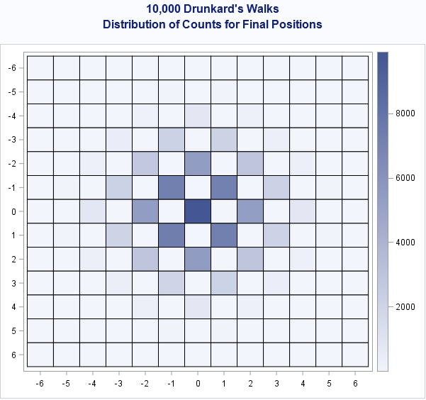
The heat map estimates the probability distribution of the final position of the drunkard after taking six steps. Notice that the drunkard must land on a spot that is an even number of units (in the Minkowski metric) from the origin. About 10% of the time the drunkard returned to the origin. About 7% of the time, the drunkard ends at (1,1), (-1,1), (-1,-1), or (1,-1). About 5% of the time the drunkard ends at (2,0), (0,2), (-2,0), or (0,-2). Positions that are four units away are less probable. Final positions that are six units away occurred during the simulation, but were so rare that they are barely visible in the heat map. For example, only 14 walks ended at the location (0, 6).

The drunkard's walk in two or more dimensions is a fun simulation of a discrete distribution. SAS/IML provides the necessary functionality to simulate many walks and to analyze the distribution of the results.