Since the pandemic began in 2020, the SAS IML developers have added about 50 new functions and enhancements to the SAS IML language in SAS Viya. Among these functions are new modern methods for optimization that have a simplified syntax as compared to the older 'NLP' functions that are available in SAS 9.4. This article discusses the new function for quadratic optimization, which is called the QPSOLVE subroutine. To illustrate the syntax, this article solves the isotonic regression problem that was solved previously by using the older NLPQUA function. Throughout the article, I will demonstrate the simpler syntax for the QPSOLVE subroutine, which solves quadratic programming (QP) problems.
The QPSOLVE syntax
In many ways, the syntax for the QPSOLVE subroutine is similar to the syntax for the NLPQUA subroutine, since they solve the same problem.
The quadratic programming (QP) problem is to find an n x 1 vector, c, that optimizes the quadratic polynomial
\(\frac{1}{2} \mathbf{c}' Q \mathbf{c} + \mathbf{v}' \mathbf{c} + \mbox{const}\)
subject to boundary constraints of the form L ≤ c ≤ U and subject to linear constraints of the form A*c ≤ b.
Here Q is a symmetric n x n matrix of quadratic coefficients, and
v is a n x 1 vector of linear coefficients.
The basic syntax for an unconstrained optimization is
CALL QPSOLVE(rc, c, Q, v);
In this syntax, rc and c are the output variables that are returned by the subroutine.
The required input arguments are Q and v. The constant term (which does not affect the optimization) can be appended to the end of the v vector to form an (n+1) x 1 vector.
The QPSOLVE subroutine also contains six optional arguments. It is convenient to use the keyword-value syntax to specify the optional parameters, as follows:
- Linear constraints: The A keyword enables you to specify a matrix of linear constraints. The B keyword enables you to specify the right-hand side of the linear system. The ROWSENSE keyword enables you to specify whether each row of the constraint matrix represents an equality constraint ('E'), a less-than-or-equals constraint ('L'), or a greater-than-or-equals constraint ('G').
- Boundary constraints: The L and U keywords enable you to specify constraints on the range of the domain of optimization. Missing values are used when the domain for a coordinate is unbounded.
- Options: The OPT keyword enables you to specify a vector of options for the optimization. The first element specifies whether the optimization is a minimization (opt[1] = 1) or a maximization (opt[1] = -1). The second element specifies the amount of output that the subroutine displays.
- Initial guess: The QPSOLVE subroutine does not require an initial guess for the optimal value.
Isotonic regression by using the QPSOLVE subroutine
In the isotonic regression problem, the QP problem is a minimization. We must specify liner constraints, but there are no boundary constraints. A previous article describes isotonic regression and explains how to form the Q matrix, the v vector, and the system of linear constraints. We use the same data set and read the data into SAS IML vectors:
/* SAS IML in Viya contains the QPSOLVE subroutine for quadratic optimization. https://go.documentation.sas.com/doc/en/pgmsascdc/v_049/casimllang/casimllang_common_sect305.htm */ data Have; set sashelp.class; x = Height; y = Weight; keep x y; run; proc iml; use Have; read all var {x y} into Z; close Have; /* If there are missing values, extract complete cases Z = completecases(Z, "extract"); */ n = nrow(Z); call sort(Z, 1); x = Z[,1]; /* the x values aren't used for the computation, only for plotting */ y = Z[,2]; |
The next step is to form the Q matrix, the v vector.
In general, the QP problem optimizes the polynomial
\(\frac{1}{2} \mathbf{c}' Q \mathbf{c} + \mathbf{v}' \mathbf{c} + \mbox{const}\)
subject to boundary constraints and linear constraints of the form A*c ≤ b.
For an isotonic regression, Q = 2*I, v = -2*y, and
\(\mbox{const} = \mathbf{y}' \mathbf{y}\), where y is the vector of Y values when the data are sorted by the X values. The following SAS IML code, which defines the coefficients for the quadratic polynomial, is the same as in the previous article:
/* to specify a QP, specify matrix Q and vector v and solve 1/2*b`*Q*b + v`*b + c = 0 for the vector b of parameters */ /* specify Q=2*I in three-column sparse form. (Use 2*I b/c of leading 1/2.) */ sparseQ = T(1:n) || T(1:n) || j(n,1,2); /* 2*I */ v = -2*y`; /* specify linear vector and constant term */ const = ssq(y); linvec = v || const; |
For the linear constraints A*c ≤ b, the definition of the A matrix and the b vector do not change. However, in the QPSOLVE subroutine, the "row sense" operator is a character vector with the values 'L' for '≤', 'E' for '=', and 'G' for '≥'. Also, the linear constraints and the boundary constraints are handled separately. Consequently, here's how you define the linear constraints:
/* Specify the linear inequalities as a matrix system. For an increasing isotonic model, A*b <= 0. Use EQCode='L' for LEQ and 'G' for GEQ. For QPSOLVE, the A matrix, the inequality symbol, and the RHS are specified separately. */ /* define subscripts of diagonal and superdiagonal elements. See https://blogs.sas.com/content/iml/2015/11/25/extract-elements-matrix.html */ A = j(n-1, n, 0); dim = dimension(A); rows = T(1:n-1); /* row numbers */ diag = rows || rows; /* (i,i) subscripts */ superDiag = rows || rows+1; /* (i,i+1) subscripts */ A[ sub2ndx(dim,diag ) ] = 1; /* +1 on diagonal */ A[ sub2ndx(dim,superDiag) ] = -1; /* -1 on superdiagonal */ /* use correlation to decide whether model is increasing or decreasing */ r = corr(Z); if r[1,2] > 0 then EQCode = 'L'; /* LE for monotone increasing */ else EQCode = 'G'; /* GE for monotone decreasing */ rowsense = j(n-1, 1, EQCode); b = j(n-1, 1, 0); /* RHS */ |
The only remaining task is to set the options for the subroutine and call the subroutine. I will use keyword-value pairs to make the calling syntax for the linear constraints easier to understand:
/* for QPSOLVE, no initial guess is required! */ optn = {1 0}; /* minimize quadratic; no print */ call QPSOLVE(rc, c, sparseQ, linvec) A=A ROWSENSE=rowsense B=b OPT=optn; pred = c; /* write to SAS data set and plot result */ create want var{'x' 'y' 'pred'}; append; close; QUIT; title "Isotonic Regression"; proc sgplot data=Want noautolegend; scatter x=x y=y; step x=x y=pred / markers markerattrs=(symbol=x) JUSTIFY=center lineattrs=GraphData2 curvelabel="Isotonic Reg"; yaxis label="y"; run; |
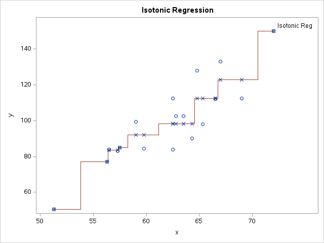
The solution vector is the same as in the previous article. The solution corresponds to a piecewise constant step function that is nondecreasing. As mentioned in the previous article, you can connect the predicted values by using any nondecreasing function. For example, a piecewise linear function is also an acceptable solution to the isotonic regression problem.
Summary
This article compares the newer QPSOLVE subroutine in SAS IML in SAS Viya to the older NLPQUA subroutine. In SAS 9.4, only the NLPQUA subroutine is available. In SAS Viya, the IML procedure and the IML action support the QPSOLVE subroutine, which has a simplified syntax and uses more modern algorithms for solving the QP problem. Whereas the older NLPQUA subroutine couples the boundary constraints and linear constraints into one matrix, the QPSOLVE subroutines handles these matrices and vectors separately by using keyword-value pairs.
