Create an interpolating polynomial in SAS

While reviewing a book on numerical analysis, I was reminded of a classic interpolation problem. Suppose you have n pairs of points in the plane: (x1,y1), (x2,y2), ..., (xn,yn), where the first coordinates are distinct. Then you can construct a unique polynomial of degree (at most) n-1 that passes through all points. The polynomial is called an interpolating polynomial. In symbols, if the polynomial is p, then p(x_k) = y_k for all k.

There are two standard constructions of the interpolation polynomial. One construction uses Lagrange polynomials. The other involves solving a matrix equation that involves a Vandermonde matrix. This article demonstrates how to construct the interpolating polynomial for n planar points by solving a linear equation.

The Vandermonde matrix

There are several ways to define a square Vandermonde matrix. A Vandermonde matrix is always defined in terms of a column vector of n values x = (x1,x2,...,xn). The most common definition uses the elementwise powers of the elements as columns of the matrix. The first column is x⁰, which is a column of 1s. The second column is x itself. The third column is x², which contains the squared elements of x. The last column is x^n-1. In general, the (i,j)th element is x_i^j-1:

$V = \begin{bmatrix} 1 & x_1 & x_1^2 & \dots & x_1^{n-1} \\ 1 & x_2 & x_2^2 & \dots & x_2^{n-1} \\ 1 & x_3 & x_3^2 & \dots & x_3^{n-1} \\ \vdots & \vdots & \vdots & \ddots & \vdots \\ 1 & x_n & x_n^2 & \dots & x_n^{n-1} \end{bmatrix}$

The Vandermonde matrix enables you to find the coefficients of the polynomial for which p(x_k) = y_k for all k. If the polynomial is $p(x) = b_0 + b_1x + b_2x^2 + \ldots + b_nx^{n-1},$ then you can find the vector of coefficients by solving the linear Vandermonde system of equations

$\begin{bmatrix} 1 & x_1 & x_1^2 & \dots & x_1^{n-1} \\ 1 & x_2 & x_2^2 & \dots & x_2^{n-1} \\ 1 & x_3 & x_3^2 & \dots & x_3^{n-1} \\ \vdots & \vdots & \vdots & \ddots & \vdots \\ 1 & x_n & x_n^2 & \dots & x_n^{n-1} \end{bmatrix} \begin{bmatrix} b_0 \\ b_1 \\ b_2 \\ \vdots \\ b_{n-1} \end{bmatrix} = \begin{bmatrix} y_1 \\ y_2 \\ y_3 \\ \vdots \\ y_n \end{bmatrix}$

If the $x_k$ are distinct, then this system has a unique solution.

An example of an interpolating polynomial

Let's use the SAS IML matrix language to define a Vandermonde matrix and to solve the Vandermonde system. Suppose you have the following five points in the plane:
(0, 5), (1, 3), (2, 0), (3, 2), (4, 1)
and you want to construct an interpolating polynomial of degree 4 that passes through each point. The following SAS IML program defines a function that returns the Vandermonde matrix from the x coordinates of the points. It then uses the SOLVE function to solve the linear system. It then prints the polynomial coefficients:

proc iml;
/* Given a vector x = {x1, x2, x3, ..., xn}, this function returns 
   the Vandermonde matrix defined by
   [ 1   x1  x1^2 ... x1^{n-1} ]
   [ 1   x2  x2^2 ... x2^{n-1} ]
   [ 1   x3  x3^2 ... x3^{n-1} ]
   [ ... ... ...  ... ...      ]
   [ 1   xn  xn^2 ... xn^{n-1} ]
*/
start Vandermonde( _x );
   x = colvec(_x);
   m = nrow(x);
   V = j(m,m,1);
   do i = 2 to m;
      V[,i] = V[,i-1] # x;
   end;
   return ( V );
finish;
 
/* Define ordered pairs. Extract the x and y coordinates */
z = {0  5,
     1  3,
     2  0,
     3  2,
     4  1};
x = z[,1];
y = z[,2];
 
/* create the Vandermonde matrix for the x; solve the system */
V = Vandermonde(x);
b = solve(V, y);
print b[r=('b0':'b5')];;

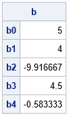
The result is that the interpolating polynomial has the equation $p(x) = 5 + 4 x - 9.916 x^2 + 4.5 x^3 - 0.583 x^4,$

Evaluating the interpolating polynomial at other points

A previous article shows how to use Horner's method to evaluate a polynomial efficiently. The SAS IML function from that article, Polyval, is reproduced below. However, the function assumes that the coefficients are sorted in decreasing order by the degree of the polynomial. Because the coefficients in the previous section are sorted in increasing order, we must reverse the vector of coefficients before calling the function. The following IML statements evaluate the fourth-degree polynomial on a regular grid. The original points and the graph of the polynomial are then written to a SAS data set and plotted by using PROC SGPLOT:

/* Polyval(c,x) uses Horner's scheme to return the value of a polynomial of 
   degree n evaluated at x. The input argument c is a column 
   vector of length n+1 whose elements are the coefficients 
   in descending powers of the polynomial to be evaluated.
   The input argument x can be a vector of values. 
   See https://blogs.sas.com/content/iml/2011/09/14/evaluate-polynomials-efficiently-by-using-horners-scheme.html
*/
start Polyval(coef, _x);
   c = colvec(coef); x = colvec(_x); /* make column vectors */
   y = j(nrow(x), 1, c[1]); /* initialize to c[1] */
   do j = 2 to nrow(c); 
      y = y # x + c[j];
   end;
   return(y);
finish;
 
/* to use the Polyval function, reverse the order of c */
c = b[nrow(b):1];
 
/* evaluate polynomial on regular grid on[min(x), max(x)] */
t = T( do(min(x), max(x), (max(x)-min(x))/100) );
f = Polyval(c,t);
create Out from z t f[c={'x' 'y' 't' 'interp'}];
append from z t f;
close;
quit;
 
title "Interpolating Polynomial";
proc sgplot data=Out;
   scatter x=x y=y;
   series x=t y=interp;
   xaxis grid;
   yaxis grid;
run;

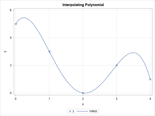
The graph of the polynomial shows that it passes through the five data points.

Summary

This article shows how to construct an interpolating polynomial of degree (at most) n-1 that passes through n planar points that have distinct x values. The technique constructs a Vandermonde matrix from the distinct x values. It then solves a linear system to obtain the coefficients of the interpolating polynomial. To visualize the graph of the polynomial, you can use Horner's method to evaluate the polynomial on a regular grid.

Blogs