Many well-known distributions become more and more "normal looking" for large values of a parameter. Famously, the binomial distribution, Binom(p, N), can be approximated by a normal distribution when N (the sample size) is large. Similarly, the Poisson(λ) distribution is well approximated by the normal distribution when λ is large.

So it is with the distribution of the sum of n six-sided dice. For n=1 die, the probability distribution is uniform. For n=2 dice, the probability distribution of the sum is triangular with a peak at sum=7. The distributions of the sum of three or more dice have been known for at least a hundred years and can be derived in several ways. This article computes the distribution of the sum of n dice for any value of n by using a formula that involves the sum of certain binomial coefficients. The formula appears in several places, including the MathWorld article about dice (Eqn 10). An early reference is J. V. Uspensky's textbook from 1937.

A formula for the distribution of n six-sided dice

A binomial coefficient counts the number of ways that you can choose j items from among a set of k items, so the binomial coefficients often appear in computations of discrete probabilities. See the MathWorld article for the derivation. Let Y be the random variable for the sum of rolling n six-sided dice. The probability that the sum of n six-sided die is Y=y is given by the following formula:

$$P(Y=y|n) = {\frac {1}{6^n}} \sum _{i=0}^M (-1)^i {n \choose i} {y-6i-1 \choose n-1}$$

For n six-sided dice, the smallest possible sum is n, which happens only when all dice equal 1. Similarly, the largest possible sum is 6*n, which happens when all dice equal 6. For any other sums, the probability is 0. Thus, the support of the distribution is the set of integers in [n, 6n].

You can implement this formula by using the SAS DATA step. Notice the DO loop in which Y (the sum) starts at n and ends at 6*n. That is the loop that computes the probability of each sum. The probability requires a summation (DO loop) for i=0..M.

data ProbDice;
keep n y cnt p;
label y="Sum of Dice"
      n="Number of Dice Rolled"
      cnt="Count of Number of Ways to Obtain Sum"
      p="Probability of Sum";
do n = 1 to 10;
   do y = n to 6*n;
      cnt = 0;
      M = floor((y-n)/6);   /* upper limit of summation */
      do i=0 to M;
         sgn = ifn( mod(i,2)=0, 1, -1 ); /* = (-1)^i */
         cnt = cnt + sgn * comb(n,i)*comb(y-6*i-1, n-1);
      end;
      p = cnt / 6**n;
      output;
   end;
end;
run;

The conversion from the formula to SAS code is straightforward. I use the MOD function instead of (-1)ⁱ because the MOD function is more efficient. Two built-in SAS functions are useful: the FLOOR function for integer truncation, and the COMB function for the number of combinations. I could have set n to be a constant, but instead I applied the formula for n=1, 2, 3, ..., 10.

Let's visualize a few of the discrete distributions by using a needle plot:

title "Probability of the Sum of n Dice";
proc sgpanel data=ProbDice;
where n in (1,2,3,5,10) and p > 1E-4;    /* omit tiny and zero-probability events */
   panelby n / onepanel columns=1;
   needle x=y y=p / markers;
   rowaxis grid;
   colaxis grid;
run;

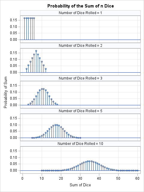
The graph shows the following distributions:

• n=1: The distribution is uniform. For one die, the numbers 1-6 appear with equal probability 1/6.
• n=2: The distribution is the familiar triangular distribution where the sums 2 and 12 appear least often, and 7 is the sum that appears most frequently.
• n=3: The distribution is looking slightly bell-shaped. The sums 3 and 18 appear least often, and 10 and 11 are the sums with the highest probability.
• n=5: The distribution is looking more bell-shaped with expected value 3.5*5 = 17.5. The sums 5 and 30 appear least often, and 17 and 18 are the sums with the highest probability.
• n=10: The distribution is looking very bell-shaped with expected value 3.5*10 = 35. The sums 10 and 60 appear rarely.

If you want to plot only one of the distributions, you can use the following call to PROC SGPLOT:

/* visualize one distribution, such as n=3 */
title "Probability of the Sum of n=3 Dice";
proc sgplot data=ProbDice;
where n = 3 and p > 1E-4;    /* omit tiny and zero-probability events */
   needle x=y y=p / markers;
   xaxis grid;
   yaxis grid;
run;

Using the distribution to compute probabilities

What is the probability that the sum of n=5 six-sided dice is less than 10? Or that the sum is greater than 20? You can use the distribution for n=5 to answer question like this. The data set ProbDice contains the discrete distributions for n=1..10, so the first step is to use a WHERE clause to restrict the data to n=5. The next step is to accumulate (add up) all the probabilities less the specified value. This gives the left-tail probability P(Y < y). If you want a right-tailed probability, you can reverse the inequality. For example, the next call to PROC MEANS outputs the probability that the sum is less than 10. The second call computes the probability that the sum is greater than 20:

ods noproctitle;   /* suppress procedure names */
/* probability that sum < 10? */
title "P(y < 10)";
proc means data=ProbDice sum nolabels;
   where n=5 and y < 10;
   var p;
run;
 
/* probability that sum > 20? */
title "P(y > 20)";
proc means data=ProbDice sum nolabels;
   where n=5 and y > 20;
   var p;
run;

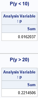
The output shows that if you roll five six-side dice, there is a 1.6% chance that the sum of the dice is less than 10. There is a 22.1% chance that the sum is greater than 20.

Summary

This article shows a classic formula for the sum of n six-side dice. You can translate the formula into SAS and use the DATA step to compute the exact distribution for any value of n. You can use PROC SGPLOT to visualize one distribution, or use PROC SGPANEL to display a panel of distributions. You can sum the individual probabilities to obtain the probability that the sum is less than or greater than some value.

As shown on the MathWorld website, you can replace the number 6 by another number, s, (such as s=4 or s=10), to obtain the distributions of n s-sided dice.