On a SAS discussion forum, a statistical programmer asked about how to understand the statistics that are displayed when you use the TEST statement in PROC REG (or other SAS regression procedures) to test for linear relationships between regression coefficients. The documentation for the TEST statement in PROC REG explains the F test in terms of a matrix of linear constraints. However, the programmer wanted a simpler explanation.
Fortunately, there is an easy way to explain the TEST statement from first principles. The explanation involves running two regression models. The first is the "full model," and the second is a "reduced model." The reduced model enforces the parameter relationships that you specify on the TEST statement. By using the ANOVA tables of the full and reduced models, you can reconstruct the F test that is displayed by the TEST statement.
This article shows two examples that reproduce and explain the results of the TEST statement. The first example is a simple linear regression, which means there is one explanatory variable. If you test whether the slope coefficient is 0, the reduced model is the intercept-only model. The second example is more complicated and involves specifying a relationship between three regression coefficients in a multivariate regression.
For a mathematical description of the F test, see the Penn State online course notes for the general linear F test.
Simulate data from a regression model
The TEST statement enables you to infer whether the regression parameters for a population satisfy some
specified relationships. A good way to understand regression is to use simulation to generate a random sample from a known regression model. For example, the following DATA step generates a sample of size 100 for which
y = 17 + 2*x1 + 0*x2 + 3*x3 + ε
where ε ~ N(0,30) is a random error term. For this sample, the correctly specified model should have parameter estimates that are close to the values β = (17, 2, 0, 3) and have a root-mean-square error (RMSE) close to 30. Furthermore, the model satisfies the linear constraints
β2 = 0 and
β3 + β1 = 5.
%let N = 100; data Full; call streaminit(123); do i = 1 to &N; x1 = rand("Normal", 25, 5); x2 = rand("Normal", 14, 2); x3 = rand("Normal", 40, 9); eps = rand("normal", 0, 30); y = 17 + 2*x1 + 0*x2 + 3*x3 + eps; output; end; keep x1-x3 y; run; |
The TEST statement for a simple linear regression
Before exploring a model that has three variables, let's look at a simple one-regressor model:
y = β0 + β2*x2 + ε
/* simple regression = one explanatory variable */ proc reg data=Full plots=none; Simple: model y = x2; H0: test x2=0; /* reduced model is intercept-only model */ ods select ANOVA TestANOVA; run; |
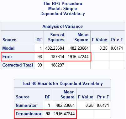
The first table is the ANOVA table for the full model. This table shows how well the model predicts the response variable. The "Error" row contains the residual sum of squares (RSS) for the full model. The last row contains the RSS for the intercept-only model. The DF and "Sum of Squares" in the first row are found by subtracting the second row from the third.
The second table is called the TestANOVA table. The TestANOVA table contains statistics related to the hypothesis test. The test statistic is an F statistic. As expected, for these data, the F statistic is small. Accordingly, the test fails to reject the null hypothesis. (And we know that β2=0 for these simulated data.) The important fact that I want to point out is that the "Denominator" row in the TestANOVA table is a copy of the "Error" row in the ANOVA table for the full mode. That fact remains true when we consider multivariate regression models.
For a one-variable regression model and for the null hypothesis β2=0, the reduced model happens to be intercept-only model. Therefore, in this situation, the first row ("Numerator") of the TestANOVA table contains the same information as the first row ("Model") of the ANOVA table. However, as we will see in the next section, this result does not hold in general.
The TEST statement for a multivariate linear regression
We can run the F test for the null hypothesis that β2 = 0 and β3 + β1 = 5. Because we know the true model for these simulated data, we expect that the F test will fail to reject the null hypothesis.
proc reg data=Full plots=none; Full: model y = x1 x2 x3; H0: test x1+x3=5, x2=0; ods select ANOVA TestANOVA; ods output ANOVA=ANOVA_Full; /* save ANOVA table for full model */ quit; |
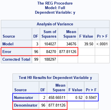
As before, the "Denominator" row of the TestANOVA table is the same as the "Error" row of the ANOVA table for the full model. However, the "Numerator" row for this null hypothesis does not appear in any other output table. The "Numerator" row corresponds to the RSS for the reduced model, which is the model that you get when you restrict the regression coefficients to the values on the TEST statement. But how can we get that information from PROC REG?
One way is to explicitly construct the reduced model by enforcing the constraints on the regression coefficients.
The unconstrained model is
y = β0 + β1 x1 + β2 x2 + β3 x3 + ε
If you impose the constraints β2 = 0 and
β3 + β1 = 5, you can rewrite the regression model as
y = β0 + (5 - β3) x1 + β3 x3 + ε
Define the new variables z = y - 5*x1 and v = x3 - x1. By renaming the parameters, you get a new regression
model
z = β0 + c v + ε
data Reduced; set Full; z = y - 5*x1; /* response variable for reduced model */ v = x3 - x1; /* explanatory variable for reduced model */ run; proc reg data=Reduced plots=none; Reduced: model z = v; ods select ANOVA; ods output ANOVA=ANOVA_Red; /* save ANOVA table for reduced model */ quit; |
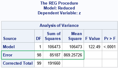
The ANOVA table for the reduced model provides the missing information that helps us to understand the statistics in the TestANOVA table. Recall that the TestANOVA table shows the F test for the full data and the linear hypothesis that β2 = 0 and β3 + β1 = 5. We can construct the F test by using the ANOVA table for the reduced model and for the full model.
Create the F test manually
The Penn State online course notes show how to construct an F test by using the "Error" rows of the ANOVA tables for the full and reduced model. Define RSSF to be the residual sum of squares for the full model, and let DFF be the error degrees of freedom for the full model. Similarly, define RSSR to be the RSS for the reduced model and let DFR be the error degrees of freedom. Then you can define MNum = (RSSR - RSSF) / (DFR - DFF) and MDenom = RSSF / DFF. The F statistic is the ratio F = MNum / MDenom.
PROC REG stored the ANOVA tables for both models in data sets. You can read the data into a DATA step or into PROC IML and construct the F test manually:
proc iml; use ANOVA_Full where(Source="Error"); read all var {"DF" "SS"} into Full[c=varNames]; close; use ANOVA_Red where(Source="Error"); read all var {"DF" "SS"} into Red[c=varNames]; close; DF_Num = Red['DF'] - Full['DF']; /* or use Red[1] - Full[1] */ RSS_Num = Red['SS'] - Full['SS']; /* or use Red[2] - Full[2], etc */ DF_Denom = Full['DF']; RSS_Denom = Full['SS']; MS_Num = RSS_Num / DF_Num; MS_Denom = RSS_Denom / DF_Denom; F = MS_Num / MS_Denom; /* F statistic for test */ pVal = sdf("F", F, DF_Num, DF_Denom); /* p-value = 1 - CDF('F', F, DF_Num, DF_Denom) */ TestTable = (DF_Num || RSS_Num || MS_Num || F || pVal) // (DF_Denom|| RSS_Denom|| MS_Denom|| . || .); print TestTable[r={'Numerator' 'Denominator'} c={'DF' 'RSS' 'Mean Sq' 'F Value' 'Pr > F'}]; |
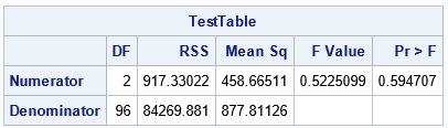
Compare this table to the TestANOVA table in the previous section. This output reproduces the TestANOVA table that PROC REG produced automatically. For clarity, I added columns for the RSS. The DF and RSS statistics in the first row are the difference between the DF and RSS statistics in the reduced and full models.
Summary
You can understand the F test for linear hypotheses in regression models by looking at the ANOVA tables for the full and reduced models. The "reduced model" is the regression model after constraining the parameters according to the null hypothesis. The ANOVA tables for the full and reduced models contain information about the residual sum of squares (RSS). You can use the differences between the reduced and full models to construct the F test for linear hypotheses. The F test is computed automatically in PROC REG (and other SAS regression procedures) by using the TEST statement. However, this article shows how to manually produce the F test by using PROC REG in SAS to explicitly evaluate the full and reduced models. The manual computation shows how the statistics produced by the TEST statement are related to the ANOVA for the full and reduced models.
