Here's a fun problem to think about: Suppose that you have two different valid ways to test a statistical hypothesis. For a given sample, will both tests reject or fail to reject the hypothesis? Or might one test reject it whereas the other does not?

The answer is that two different tests can and will disagree for some samples, although they are likely to agree most of the time. Statistical software sometimes displays the results of multiple statistical tests when you request a hypothesis test. For example, PROC UNIVARIATE in SAS outputs four different statistical tests for normality, including the Shapiro-Wilk and Kolmogorov-Smirnov tests. One or more tests might reject the hypothesis of normality whereas other tests fail to reject it.

A SAS customer asked a question that made me wonder how often the four normality tests agree, and what the samples look like when the tests do not agree. This article presents a simulation study that generates random samples from the normal distribution and calls PROC UNIVARIATE to perform tests for normality on each sample. At the 95% confidence level, we expect each of these tests to reject the test of normality for 5% of the samples. But even though the tests all are designed to detect normal data, they do so in different ways. This means that the 5% of samples that are rejected by one test might be different from the 5% of samples that are rejected by another test.

Tests for Normality

PROC UNIVARIATE in SAS supports four different tests for normality of a univariate distribution. The Shapiro-Wilk statistic (W) is based on a computation that involves the variance and quantiles of the data. The other three tests are based on the empirical cumulative distribution function (ECDF). The ECDF-based tests include the Kolmogorov-Smirnov statistic (D), the Anderson-Darling statistic (A²), and the Cramer–von Mises statistic (W²). When the associate p-value of a statistic is less than α, the test rejects the null hypothesis ("the sample is from a normal distribution") at the α significance level. This article uses α=0.05.

What should an analyst do if some tests reject the hypothesis whereas others fail to reject it? I know a statistician who habitually rejects the assumption of normality if ANY of the tests reject normality. I think this is a bad idea because he is making decisions at less than the 95% confidence level. The simulation study in this article estimates the probability that a random sample from the normal distribution is not rejected simultaneously by all four tests. That is, all four tests agree that the sample is normal.

Run a simulation study

If you simulate a moderate-sized sample from the normal distribution, these four tests should each reject normality for about 5% of the samples. The following SAS program uses the standard Monte Carlo simulation technique in SAS:

1. Simulate B=10,000 samples of size N=50 from the normal distribution. Associate a unique ID to each sample.
2. Make sure that you suppress the output. Then use the BY statement to analyze the B samples. Write the B statistics to a data set.
3. Analyze the sampling distribution of the statistics or tabulate the results of a statistical test.

The first two steps are straightforward. You can use the ODS OUTPUT statement to save the statistics to a data set, as follows:

/* simulate normal data */
%let n = 50;
%let numSamples = 10000;
data Sim;
call streaminit(123);
do SampleID=1 to &NumSamples;
   do i = 1 to &n;
      x = rand("Normal", 0);  /* sample from null hypothesis */
      output;
   end;
end;
run;
 
ods exclude all;    /* suppress output */
proc univariate data=Sim normal;
   by SampleID;
   var x;
   ods output TestsForNormality = NormTests;
run;
ods exclude none;

Transpose and analyze the results of the simulation study

The TestsForNormality table lists the statistics in a "long form," where each statistic is on a separate row. To analyze the distribution of the statistics, it is convenient to transpose the data to wide form. The following call to PROC TRANSPOSE creates four variables (pValue_W, pValue_D, pValue_W_Sq, and pValue_A_Sq), which are the p-values for the four normality tests.

/* Transpose from long to wide form. This creates four variables
   pValue_W, pValue_D, pValue_W_Sq, and pValue_A_Sq. */
proc transpose data=NormTests out=Tran prefix=pValue_;
   by SampleID;
   id TestLab;
   var pValue;
run;

Let's create a binary indicator variable for each p-value. The indicator variable has the value 1 if the rejects the hypothesis of normality at the α=0.05 significance level. If the test fails to reject, the indicator variable has the value 0. You can then tabulate the results for each individual test:

%let alpha = 0.05;
data Results;
set Tran;
RejectW = (pValue_W < &alpha);
RejectD = (pValue_D < &alpha);
RejectWSq = (pValue_W_Sq < &alpha);
RejectASq = (pValue_A_Sq < &alpha);
run;
 
/* tabulate the results */
proc freq data=Results;
   tables RejectW RejectD RejectWSq RejectASq / norow nocol nocum;
run;

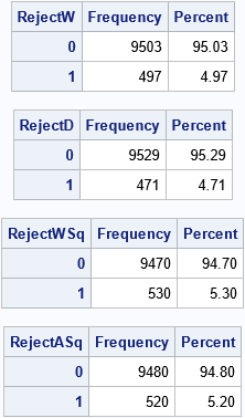
As expected, each test rejects the hypothesis of normality on about 5% of the random samples. However, the tests have different characteristics. For a given sample, one test might reject the hypothesis whereas another test fails to reject it. For example, you can investigate how many samples were jointly rejected by the Shapiro-Wilk test (W) and the Kolmogorov-Smirnov test (D):

proc freq data=Results;
   tables RejectW*RejectD / norow nocol nocum list; 
run;

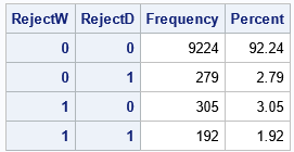
The table shows the results of 10,000 statistical tests. For 192 samples (1.9%), both reject the null hypothesis. For 9,224 (92.2%) samples, both tests fail to reject it. Thus the tests agree for 9,416 samples or 94.2%.

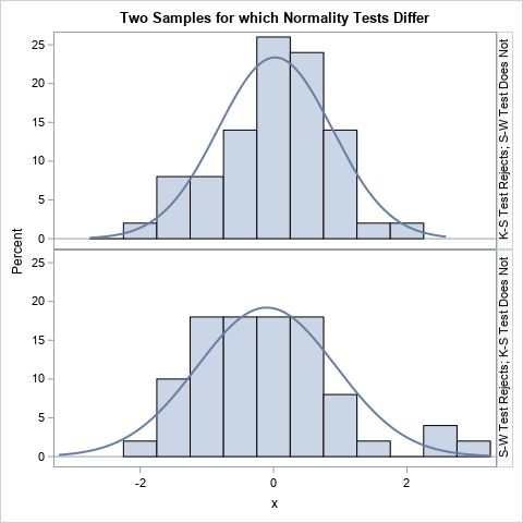
The interesting cases are when one test rejects the hypothesis and the other does not. The Kolmogorov-Smirnov test rejects the hypothesis on 279 samples that are not rejected by the Shapiro-Wilk test. Conversely, the Shapiro-Wilk test rejects 305 samples that the Kolmogorov-Smirnov test does not reject. Two such samples are shown in the following graph. A casual inspection does not reveal why the tests differ on these samples, but they do.

Multiple tests

When you run four tests, the situation becomes more complicated. For a given sample, you could find that zero, one, two, three, or all four tests reject normality. Since these statistics all test the same hypothesis, they should agree often. Thus, you should expect that for most random samples, either zero or four tests will reject the null hypothesis. Again, the interesting cases are when some tests reject it and others fail to reject it. The following table shows the results of all four tests on the samples in the simulation study:

 
proc freq data=Results;
   tables RejectW*RejectD*RejectWSq*RejectASq / norow nocol nocum list;
run;

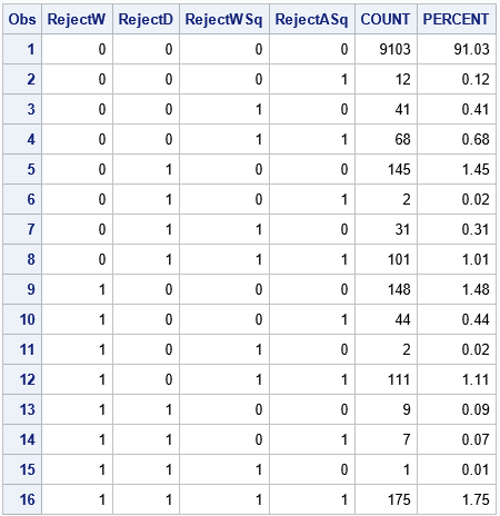
There are a total of 9,103 samples for which all tests agree that the sample is normally distributed. If you reject the hypothesis if ANY of the tests reject it, you are making decisions at the 91% confidence level, not at the 95% level.

The first and last rows show the cases where all four tests agree. You can see that the tests agree with each other about 92.8% of the time. However, there are some other cases that occur frequently:

• The 5th and 12th rows indicate samples for which the Kolmogorov-Smirnov test does not agree with the other three tests. This happens for 2.6% of the samples.
• The 8th and 9th rows indicate samples for which the Shapiro-Wilk test does not agree with the ECDF tests. This happens for 2.5% of the samples.
• The ECDF tests agree with each other for 95.3% of these samples. This is shown by the 1st, 8th, 9th, and 16th rows.
• It is very rare for the Anderson-Darling statistic (A²) and the Cramer–von Mises statistic (W²) to disagree when the null hypothesis is true. They agree for 98.6% of these samples.

Summary

This article uses a simulation study to investigate how often different tests (for the same hypothesis) agree with each other. The article uses small samples of size N=50 that are normally distributed. The results show that these tests for normality tend to agree with each other. At least one test disagrees with the others for 7.2% of the samples.

As usual, this simulation study applies only to the conditions in the study. Wicklin (Simulating Data with SAS, 2013, p. 105) cautions against generalizing too much from a particular simulation: "real data are rarely distributed according to any 'named' distribution, so how well do the results generalize to real data? The answer can depend on the true distribution of the data and the sample size."

Nevertheless, this article provides some insight into how often statistical tests of normality agree and disagree with each other when the null hypothesis is true. You can use the techniques in this article to compare other tests.