A quadratic form is a second-degree polynomial that does not have any linear or constant terms. For multivariate polynomials, you can quickly evaluate a quadratic form by using the matrix expression
x` A x
This computation is straightforward in a matrix language such as SAS/IML. However, some computations in statistics require that you evaluate a quadratic form that looks like
x` A^-1 x
where A is symmetric and positive definite. Typically, you know A, but not the inverse of A. This article shows how to compute both kinds of quadratic forms efficiently.

What is a quadratic form?

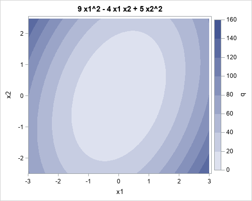
For multivariate polynomials, you can represent the purely quadratic terms by a symmetric matrix, A. The polynomial is q(x) = x` A x, where x is an d x 1 vector and A is a d x d symmetric matrix. For example, if A is the matrix {9 -2, -2 5} and x = {x1, x2} is a column vector, the expression x` A x equals the second degree polynomial q(x1, x2) = 9*x1² - 4*x1 x2 + 5*x2². A contour plot of this polynomial is shown below.

Probably the most familiar quadratic form is the squared Euclidean distance. If you let A be the d-dimensional identity matrix, then the squared Euclidean distance of a vector x from the origin is x` I<sub>d</sub> x = x` x = Σ_i x_i². You can obtain a weighted squared distance by using a diagonal matrix that has positive values. For example, if W = diag({2, 4}), then x` W x = 2*x1² + 4*x2². If you add in off-diagonal elements, you get cross terms in the polynomial.

Efficient evaluation of a quadratic form

If the matrix A is dense, then you can use matrix multiplication to evaluate the quadratic form. The following symmetric 3 x 3 matrix defines a quadratic polynomial in 3 variables. The multiplication evaluates the polynomial at (x1, x2, x3) = (-1. 2. 0.5).

proc iml;
/* 
   q(x1, x2, x3) = 4*x1**2 + 6*x2**2 + 9*x3**2 +
                   2*3*x1*x2 + 2*2*x1*x3 + 2*1*x2*x3
*/
A = {4 3 2,
     3 6 1,
     2 1 9};
x = {-1, 2, 0.5};
q1 = x`*A*x;
print q1;

When you are dealing with large matrices, always remember that you should never explicitly form a large diagonal matrix. Multiplying with a large diagonal matrix is a waste of time and memory. Instead, you can use elementwise multiplication to evaluate the quadratic form more efficiently:

w = {4, 6, 9};
q2 = x`*(w#x);     /* more efficient than q = x`*diag(w)*x; */
print q2;

Quadratic forms with positive definite matrices

In statistics, the matrix is often symmetric positive definite (SPD). The matrix A might be a covariance matrix (for a nondegenerate system), the inverse of a covariance matrix, or the Hessian evaluated at the minimum of a function. (Recall that the inverse of a symmetric positive definite (SPD) matrix is SPD.) An important example is the squared Mahalanobis distance x` Σ^-1 x, which is a quadratic form.

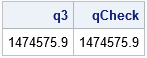
As I have previously written, you can use a trick in linear algebra to efficiently compute the Mahalanobis distance. The trick is to compute the Cholesky decomposition of the SPD matrix. I'll use a large Toeplitz matrix, which is guaranteed to be symmetric and positive definite, to demonstrate the technique. The function EvalSPDQuadForm evaluates a quadratic form defined by the SPD matrix A at the coordinates given by x:

/* Evaluate quadratic form q = x`*A*x, where A is symmetric positive definite.
   Let A = U`*U be the Cholesky decomposition of A.
   Then q = x`(U`*U)*x = (U*x)`(Ux)
   So define z = U*x and compute q = z`*z
*/
start EvalSPDQuadForm(A, x);
   U = root(A);           /* Cholesky root */
   z = U*x;
   return (z` * z);       /* dot product of vectors */
finish;
 
/* Run on large example */
call randseed(123);
N = 1000;
A = toeplitz(N:1);
x = randfun(N, "Normal");
 
q3 = EvalSPDQuadForm(A, x);  /* efficient */
qCheck = x`*A*x;             /* check computation by using a slower method */
 
print q3 qCheck;

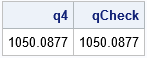
You can use a similar trick to evaluate the quadratic form x` A^-1 x. I previously used this trick to evaluate the Mahalanobis distance efficiently. It combines a Cholesky decomposition (the ROOT function in SAS/IML) and the TRISOLV function for solving triangular systems.

/* Evaluate quadratic form x`*inv(A)*x, where  A is symmetric positive definite.
   Let w be the solution of A*w = x and A=U`U be the Cholesky decomposition.
   To compute  q = x` * inv(A) * x = x` * w, you need to solve for w.
   (U`U)*w = x, so
        First solve triangular system U` z = x   for z,
        then solve triangular system  U w = z   for w 
*/
start EvalInvQuadForm(A, x);
   U = root(A);              /* Cholesky root */
   z = trisolv(2, U, x);     /* solve linear system */
   w = trisolv(1, U, z);  
   return (x` * w);          /* dot product of vectors */
finish;
 
/* test the function */
q4 = EvalInvQuadForm(A, x);  /* efficient */
qCheck = x`*Solve(A,x);      /* check computation by using a slower method */
print q4 qCheck;

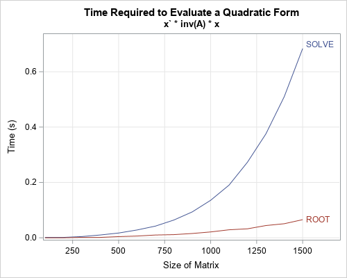
You might wonder how much time is saved by using the Cholesky root and triangular solvers, rather than by computing the general solution by using the SOLVE function. The following graph compares the average time to evaluate the same quadratic form by using both methods. You can see that for large matrices, the ROOT-TRISOLV method is many times faster than the straightforward method that uses SOLVE.

In summary, you can use several tricks in numerical linear algebra to efficiently evaluate a quadratic form, which is a multivariate quadratic polynomial that contains only second-degree terms. These techniques can greatly improve the speed of your computational programs.