In numerical linear algebra, there are often multiple ways to solve a problem, and each way is useful in various contexts. In fact, one of the challenges in matrix computations is choosing from among different algorithms, which often vary in their use of memory, data access, and speed. This article describes four ways to perform the sum of squares and crossproducts matrix, which is usually abbreviated as the SSCP matrix. The SSCP matrix is an essential matrix in ordinary least squares (OLS) regression. The normal equations for OLS are written as (X`*X)*b = X`*Y, where X is a design matrix, Y is the vector of observed responses, and b is the vector of parameter estimates, which must be computed. The X`*X matrix (pronounced "X-prime-X") is the SSCP matrix and the topic of this article.

If you are performing a least squares regressions of "long" data (many observations but few variables), forming the SSCP matrix consumes most of the computational effort. In fact, the PROC REG documentation points out that for long data "you can save 99% of the CPU time by reusing the SSCP matrix rather than recomputing it." That is because the SSCP matrix for an n x p data matrix is a symmetric p x p matrix. When n ≫ p, forming the SSCP matrix requires computing with a lot of rows. After it is formed, it is relatively simple to solve a p x p linear system.

SSCP as a matrix computation

Conceptually, the simplest way to compute the SSCP matrix is by multiplying the matrices in an efficient manner. This is what the SAS/IML matrix language does. It recognizes that X`*X is a special kind of matrix multiplication and uses an efficient algorithm to form the product. However, this approach requires that you be able to hold the entire data matrix in RAM, which might not be possible when you have billions of rows.

The following SAS DATA Step creates a data matrix that contains 426 rows and 10 variables. The PROC IML step reads the data into a matrix and forms the SSCP matrix:

/* remove any rows that contain a missing value:
   https://blogs.sas.com/content/iml/2015/02/23/complete-cases.html */
data cars;
set sashelp.cars;
if not nmiss(of _numeric_);
run;
 
proc iml;
use cars;  read all var _NUM_ into X[c=varNames]; close;
/* If you want, you can add an intercept column: X = j(nrow(X),1,1) || X; */
n = nrow(X);
p = ncol(X);
SSCP = X`*X;         /* 1. Matrix multiplication */
print n p, SSCP;

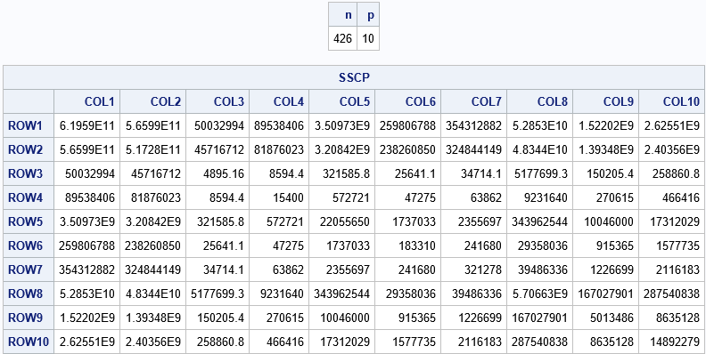
Although the data has 426 rows, it only has 10 variables. Consequentially, the SSCP matrix is a small 10 x 10 symmetric matrix. (To simplify the code, I did not add an intercept column, so technically this SSCP matrix would be used for a no-intercept regression.)

SSCP as an array of inner product computations

The (i,j)th element of the SSCP matrix is the inner product of the i_th column and the j_th column. In general, Level 1 BLAS computations (inner products) are not as efficient as Level 3 computations (matrix products). However, if you have the data variables (columns) in an array of vectors, you can compute the p(p+1)/2 elements of the SSCP matrix by using the following loops over columns. This computation assumes that you can hold at least two columns in memory at the same time:

/* 2. Compute SSCP[i,j] as an inner-product of i_th and j_th columns */
Y = j(p, p, .);
do i = 1 to p;
   u = X[,i];             /* u = i_th column */
   do j = 1 to i;
      v = X[,j];          /* v = j_th column */
      Y[i,j] = u` * v;   
      Y[j,i] = Y[i,j];    /* assign symmetric element */
   end;
end;

SSCP as a sum of outer products of rows

The third approach is to compute the SSCP matrix as a sum of outer products of rows. Before I came to SAS, I considered the outer-product method to be inferior to the other two. After all, you need to form n matrices (each p x p) and add these matrices together. This did not seem like an efficient scheme. However, when I came to SAS I learned that this method is extremely efficient for dealing with Big Data because you never need to keep more than one row of data into memory! A SAS procedure like PROC REG has to read the data anyway, so as it reads each row, it also forms outer product and updates the SSCP. When it finishes reading the data, the SSCP is fully formed and ready to solve!

I've recently been working on parallel processing, and the outer-product SSCP is ideally suited for reading and processing data in parallel. Suppose you have a grid of G computational nodes, each holding part of a massive data set. If you want to perform a linear regression on the data, each node can read its local data and form the corresponding SSCP matrix. To get the full SSCP matrix, you merely need to add the G SSCP matrices together, which are relatively small and thus cheap to pass between nodes. Consequently, any algorithm that uses the SSCP matrix can greatly benefit from a parallel environment when operating on Big Data. You can also use this scheme for streaming data.

For completeness, here is what the outer-product method looks like in SAS/IML:

/* 3. Compute SSCP as a sum of rank-1 outer products of rows */
Z = j(p, p, 0);
do i = 1 to n;
   w = X[i,];           /* Note: you could read the i_th row; no need to have all rows in memory */
   Z = Z + w` * w;
end;

For simplicity, the previous algorithm works on one row at a time. However, it can be more efficient to process multiple rows. You can easily buffer a block of k rows and perform an outer product of the partial data matrix. The value of k depends on the number of variables in the data, but typically the block size, k, is dozens or hundreds. In a procedure that reads a data set (either serially or in parallel), each operation would read k observations except, possibly, the last block, which would read the remaining observations. The following SAS/IML statements loop over blocks of k=10 observations at a time. You can use the FLOOR-MOD trick to find the total number of blocks to process, assuming you know the total number of observations:

/* 4. Compute SSCP as the sum of rank-k outer products of k rows */
/* number of blocks: https://blogs.sas.com/content/iml/2019/04/08/floor-mod-trick-items-to-groups.html */
k = 10;                                /* block size */
numBlocks = floor(n / k) + (mod(n, k) > 0);  /* FLOOR-MOD trick */
W = j(p, p, 0);
do i = 1 to numBlocks;
   idx = (1 + k*(i-1)) : min(k*i, n);  /* indices of the next block of rows to process */
   A = X[idx,];                        /* partial data matrix: k x p */
   W = W + A` * A;
end;

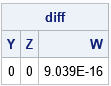
All computations result in the same SSCP matrix. The following statements compute the sum of squares of the differences between elements of X`*X (as computed by using matrix multiplication) and the other methods. The differences are zero, up to machine precision.

diff = ssq(SSCP - Y) || ssq(SSCP - Z) || ssq(SSCP - W);
if max(diff) < 1e-12 then 
   print "The SSCP matrices are equivalent.";
print diff[c={Y Z W}];

Summary

In summary, there are several ways to compute a sum of squares and crossproducts (SSCP) matrix. If you can hold the entire data in memory, a matrix multiplication is very efficient. If you can hold two variables of the data at a time, you can use the inner-product method to compute individual cells of the SSCP. Lastly, you can process one row at a time (or a block of rows) and use outer products to form the SSCP matrix without ever having to hold large amounts of data in RAM. This last method is good for Big Data, streaming data, and parallel processing of data.