I often claim that the "natural syntax" of the SAS/IML language makes it easy to implement an algorithm or statistical formula as it appears in a textbook or journal. The other day I had an opportunity to test the truth of that statement. A SAS programmer wanted to implement the conjugate gradient algorithm, which is an iterative method for solving a system of equations with certain properties. I looked up the Wikipedia article about the conjugate gradient method and saw the following text:

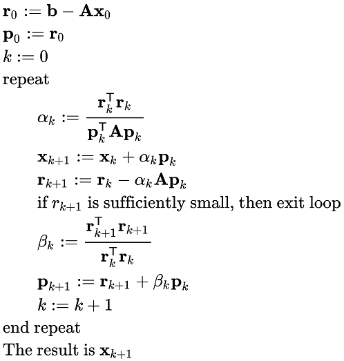
"The algorithm is detailed below for solving Ax = b where A is a real, symmetric, positive-definite matrix. The input vector x0 can be an approximate initial solution or 0." The text was accompanied by pseudocode. (In the box to the right; click to enlarge.)

The conjugate gradient method in SAS/IML

I used the pseudocode to implement the conjugate gradient method in SAS/IML. (The method is explained further in the next section.) I chose not to use the 'k' and 'k+1' notation but merely to overwrite the old values of variables with new values. In the program, the variables x, r, and p are vectors and the variable A is a matrix.

/* Linear conjugate gradient method as presented in Wikipedia:
   https://en.wikipedia.org/wiki/Conjugate_gradient_method
   Solve the linear system A*x = b, where A is a symmetric positive definite matrix.
   The algorithm converges in at most n iterations, where n is the dimension of A.
 
   This function requires an initial guess, x0, which can be the zero vector.
   The function does not verify that the matrix A is symmetric positive definite.
   This module returns a matrix mX= x1 || x2 || ... || xn 
   whose columns contain the iterative path from x0 to the approximate solution vector xn.  */
proc iml;
start ConjGrad( x0, A, b, Tolerance=1e-6 );
  x = x0;                            /* initial guess */
  r = b - A*x0;                      /* residual */
  p = r;                             /* initial direction */
  mX = j(nrow(A), nrow(A), .);       /* optional: each column is result of an iteration */
  do k = 1 to ncol(mX) until ( done );
    rpr = r`*r;  Ap = A*p;           /* store partial results */
    alpha =  rpr / (p`*Ap);          /* step size */
    x = x + alpha*p;   mX[,k] = x;   /* remember new guess */
    r = r - alpha*Ap;                /* new residual */
    done = (sqrt(rpr) < Tolerance);  /* stop if ||r|| < Tol */
    beta = (r`*r) / rpr;             /* new stepsize */
    p = r + beta*p;                  /* new direction */
  end;
  return ( mX );     /* I want to return the entire iteration history, not just x */
finish;

The SAS/IML program is easy to read and looks remarkably similar to the pseudocode in the Wikipedia article. This is in contrast to lower-level languages such as C in which the implementation looks markedly different from the pseudocode.

Convergence of the conjugate gradient method

The conjugate gradient method is an iterative method to find the solution of a linear system A*x=b, where A is a symmetric positive definite n x n matrix, b is a vector, and x is the unknown solution vector. (Recall that symmetric positive definite matrices arise naturally in statistics as the crossproduct matrix (or covariance matrix) of a set of variables.) The beauty of the conjugate gradient method is twofold: it is guaranteed to find the solution (in exact arithmetic) in at most n iterations, and it requires only simple operations, namely matrix-vector multiplications and vector additions. This makes it ideal for solving system of large sparse systems, because you can implement the algorithm without explicitly forming the coefficient matrix.

It is fun to look at how the algorithm converges from the initial guess to the final solution. The following example converges gradually, but I know of examples for which the algorithm seems to make little progress for the first n – 1 iterations, only to make a huge jump on the final iteration straight to the solution!

Recall that you can use a Toeplitz matrix to construct a symmetric positive definite matrix. The following statements define a banded Toeplitz matrix with 5 on the diagonal and specify the right-hand side of the system. The zero vector is used as an initial guess for the algorithm. The call to the ConjGrad function returns a matrix whose columns contain the iteration history for the method. For this problem, the method requires five iterations to converge, so the fifth column contains the solution vector. You can check that the solution to this system is (x1, x2, 3, x4, x5) = (-0.75, 0, 1.5, 0.5, -0.75), either by performing matrix multiplication or by using the SOLVE function in IML to compute the solution vector.

A = {5 4 3 2 1,          /* SPD Toeplitz matrix */
     4 5 4 3 2, 
     3 4 5 4 3,
     2 3 4 5 4,
     1 2 3 4 5};
b = {1, 3, 5, 4, 2};     /* right hand side */
n = ncol(A);
x0 = j(n,1,0);           /* the zero vector */
traj = ConjGrad( x0, A, b );
x = traj[ ,n];           /* for this problem, solution is in last column */

It is instructive to view how the iteration progresses from an initial guess to the final solution. One way to view the iterations is to compute the Euclidean distance between each partial solution and the final solution. You can then graph the distance between each iteration and the final solution, which decreases monotonically (Hestenes and Stiefel, 1952).

Distance = sqrt( (traj - x)[##, ] ); /* || x[j] - x_Soln || */
Iteration = 1:n;
title "Convergence of Conjugate Gradient Method";
call series(Iteration, Distance) grid={x y} xValues=Iteration 
     option="markers" label={"" "Distance to Solution"};

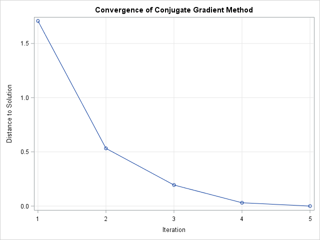
Notice in the distance graph that the fourth iteration almost equals the final solution. You can try different initial guesses to see how the guess affects the convergence.

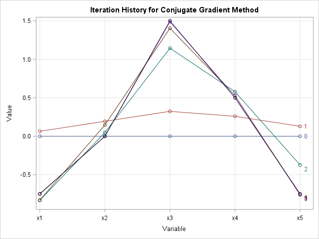
In addition to the global convergence, you can visualize the convergence in each coordinate. Because the vectors live in high-dimensional space, it impossible to draw a scatter plot of the iterative solutions. However, you can visualize each vector in "parallel coordinates" as a sequence of line segments that connect the coordinates in each variable. In the following graph, each "series plot" represents a partial solution. The curves are labeled by the iteration number. The blue horizontal line represents the initial guess (iteration 0). The partial solution after the first iteration is shown in red and so on until the final solution, which is displayed in black. You can see that the third iteration (for this example) is close to the final solution. The fourth partial solution is so close that it cannot be visually distinguished from the final solution.

In summary, this post shows that the natural syntax of the SAS/IML language makes it easy to translate pseudocode into a working program. The article focuses on the conjugate gradient method, which solves a symmetric, positive definite, linear system in at most n iterations. The article shows two ways to visualize the convergence of the iterative method to the solution.