A SAS customer asked, "I computed the eigenvectors of a matrix in SAS and in another software package. I got different answers? How do I know which answer is correct?"
I've been asked variations of this question dozens of times. The answer is usually "both answers are correct."
The mathematical root of the problem is that eigenvectors are not unique. It is easy to show this: If v is an eigenvector of the matrix A, then by definition A v = λ v for some scalar eigenvalue λ. Notice that if you define u = α v for a scalar α ≠ 0, then u is also an eigenvector because A u = α A v = α λ v = λ u. Thus a multiple of an eigenvector is also an eigenvector.
Most statistical software (including SAS) tries to partially circumvent this problem by standardizing an eigenvector to have unit length (|| v || = 1). However, note that v and -v are both eigenvectors that have the same length. Thus even a standardized eigenvector is only unique up to a ± sign, and different software might return eigenvectors that differ in sign. In fact for some problems, the same software can return different answers when run on different operating systems (Windows versus Linux), or when using vendor-supplied basic linear algebra subroutines such as the Intel Math Kernel Library (MKL).
To further complicate the issue, software might sort the eigenvalues and eigenvectors in different ways. Some software (such as MATLAB) orders eigenvalues by magnitude, which is the absolute value of the eigenvalue. Other software (such as SAS) orders eigenvalues according to the value (of the real part) of the eigenvalues. (For most statistical computations, the matrices are symmetric and positive definite (SPD). For SPD matrices, which have real nonnegative eigenvalues, these two orderings are the same.) The situation becomes more complicated if the eigenvalues are not distinct, and that case is not dealt with in this article.
Eigenvectors of an example matrix
To illustrate the fact that different software and numerical algorithms can produce different eigenvectors, let's examine the eigenvectors of the following 3 x 3 matrix:
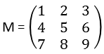
The eigenvectors of this matrix will be computed by using five different software packages: SAS, Intel's MKL, MATLAB, Mathematica, and R. The eigenvalues for this matrix are unique and are approximately 16.1, 0, and -1.1. Notice that this matrix is not positive definite, so the order of the eigenvectors will vary depending on the software. Let's compute the eigenvectors in five different ways.
Method 1: SAS/IML EIGEN Call: The following statements compute the eigenvalues and eigenvectors of M by using a built-in algorithm in SAS. This algorithm was introduced in SAS version 6 and was the default algorithm until SAS 9.4.
proc iml; reset FUZZ; /* print very small numbers as 0 */ M = {1 2 3, 4 5 6, 7 8 9}; reset EIGEN93; /* use "9.3" algorithm; no vendor BLAS (option required for SAS 9.4m3) */ call eigen(EigVal, SASEigVec, M); print EigVal, SASEigVec[colname=("E1":"E3")]; |
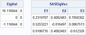
Notice that the eigenvalues are sorted by their real part, not by their magnitude. The eigenvectors are returned in a matrix. The i_th column of the matrix is an eigenvector for the i_th eigenvalue. Notice that the eigenvector for the largest eigenvalue (the first column) has all positive components. The eigenvector for the zero eigenvalue (the second column) has a negative component in the second coordinate. The eigenvector for the negative eigenvalue (the third column) has a negative component in the third coordinate.
Method 2: Intel MKL BLAS: Starting with SAS/IML 14.1, you can instruct SAS/IML to call the Intel Math Kernel Library for eigenvalue computation if you are running SAS on a computer that has the MKL installed. This feature is the default behavior in SAS/IML 14.1 (SAS 9.4m3), which is why the previous example used RESET NOEIGEN93 to get the older "9.3 and before" algorithm. The output for the following statements assumes that you are running SAS 9.4m3 or later and your computer has Intel's MKL.
reset NOEIGEN93; /* use Intel MKL, if available */ call eigen(EigVal, MKLEigVec, M); print MKLEigVec[colname=("E1":"E3")]; |
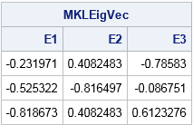
This is a different result than before, but it is still a valid set of eigenvectors The first and third eigenvectors are the negative of the eigenvectors in the previous experiment. The eigenvectors are sorted in the same order, but that is because SAS (for consistency with earlier releases) internally sorts the eigenvectors that the MKL returns.
Method 3: MATLAB: The following MATLAB statements compute the eigenvalue and eigenvectors for the same matrix:
M = [1, 2, 3; 4, 5, 6; 7, 8, 9]; [EigVec, EigVal] = eig(M); |
EigVec = -0.2320 -0.7858 0.4082 -0.5253 -0.0868 -0.8165 -0.8187 0.6123 0.4082 |
The eigenvalues are not displayed, but you can tell from the output that the eigenvalues are ordered by magnitude: 16.1, -1.1, and 0. The eigenvectors are the same as the MKL results (within rounding precision), but they are presented in a different order.
Method 4: Mathematica: This example matrix is used in the Mathematica documentation for the Eigenvectors function:
Eigenvectors[{{1, 2, 3}, {4, 5, 6}, {7, 8, 9}}] |
0.283349 -1.28335 1 0.641675 -0.141675 -2 1 1 1 |
This is a different result, but still correct. The symbolic computations in Mathematica do not standardize the eigenvectors to unit length. Instead, they standardize them to have a 1 in the last component. The eigenvalues are sorted by magnitude (like the MATLAB output), but the first column has opposite signs from the MATLAB output.
Method 5: R: The R documentation states that the eigen function in R calls the LAPACK subroutines. Thus I expect it to get the same result as MATLAB.
M <- matrix(c(1:9), nrow=3, byrow=TRUE) r <- eigen(M) r$vectors |
[,1] [,2] [,3] [1,] -0.2319707 -0.78583024 0.4082483 [2,] -0.5253221 -0.08675134 -0.8164966 [3,] -0.8186735 0.61232756 0.4082483 |
Except for rounding, this result is the same as the MATLAB output.
Summary
This article used a simple 3 x 3 matrix to demonstrate that different software packages might produce different eigenvectors for the same input matrix. There were four different answers produced, all of which are correct. This is a result of the mathematical fact that eigenvectors are not unique: any multiple of an eigenvector is also an eigenvector! Different numerical algorithms can produce different eigenvectors, and this is compounded by the fact that you can standardize and order the eigenvectors in several ways.
Although it is hard to compare eigenvectors from different software packages, it is not impossible. First, make sure that the eigenvectors are ordered the same way. (You can skip this step for symmetric positive definite matrices.) Then make sure they are standardized to unit length. If you do those two steps and the eigenvalues are distinct, then the eigenvectors will agree up to a ± sign.

6 Comments
Rick, This subject has interested me for many years since several of my procedures rely on eigenvalues and eigenvectors. Eigenvalues and eigenvectors are of course extensively used in SAS, and we want the results to be consistent across SAS releases and operating systems Options for making the results less likely to change include reflecting an eigenvectors if the sum of its elements is negative. Tied eigenvalues make the problem of reliably returning the same eigenvectors even more interesting. One easy way to create a matrix that has tied eigenvalues is to create a Hadamard matrix.
proc iml;
x = hadamard(16);
call eigen(val, vec, x);
print (val`) vec[format=5.2];
quit;
This Hadamard matrix has 8 eigenvalues equal to 4 and 8 equal to -4.
SAS has code to try to make eigenvectors unique even within large blocks of tied eigenvalues. Sometimes, algorithms will only solve for the first m eigenvalues. If eigenvalues m and m-1 are tied, then the code can optionally solve for more eigenvalues until it finds the end of the tie block so that it can then apply the code to find unique eigenvectors. Not all procedures use all of the options.
Thanks for the comments. Yes, there are additional steps you can take in an attempt to "unique-ify" the eigenvectors. Unfortunately, any linear operation is a "co-dimension 1" solution that resolves most problems but leaves others unresolved. For example, suppose there are unique eigenvalues and you decide to standardize the +/- eigenvectors by returning the one that is in the same direction as some specified vector such as e_1=(1,0,...,0). That unique-ifies most vectors, but still leaves a (p-1)-dimensional subspace ("co-dimension 1") of vectors that are orthogonal to the reference vector and therefore are not uniquely resolved. The method you mention (sum of elements positive) is a linear relationship, so suffers the same drawback.
You could, of course, start iterating: if a vector is in the orthogonal complement to e_1 you can project onto e_2=(0,1,0,...,0) for the next round, etc.
But I guess I feel like these extra steps merely make the eigenvectors more arbitrary unless every numerical software package implements the same scheme.
Pingback: Robust principal component analysis in SAS - The DO Loop
Pingback: The singular value decomposition: A fundamental technique in multivariate data analysis - The DO Loop
Do you know how the sign of each eigenvector is determined in the SAS/IML EIGEN Call algorithm?
Thanks for your help!
I wish I could, but I don't think it is possible to predict in advance which sign an algorithm will produce. The sign depends on the data as well as the numerical algorithm.