Last week I showed how to compute nearest-neighbor distances for a set of numerical observations. Nearest-neighbor distances are used in many statistical computations, including the analysis of spatial point patterns. This article describes how the distribution of nearest-neighbor distances can help you determine whether spatial data are uniformly distributed or whether they show evidence of non-uniformity such as clusters of observations. You can examine the spatial data manually or use a SAS/STAT procedure (PROC SPP) that automates common spatial analyses.

The distribution of nearest neighbor distances

The distribution of the nearest-neighbor distances provides information about the process that generated the spatial data. Let's look at two example: clustered data for trees in a forest and uniformly distributed (simulated) data.

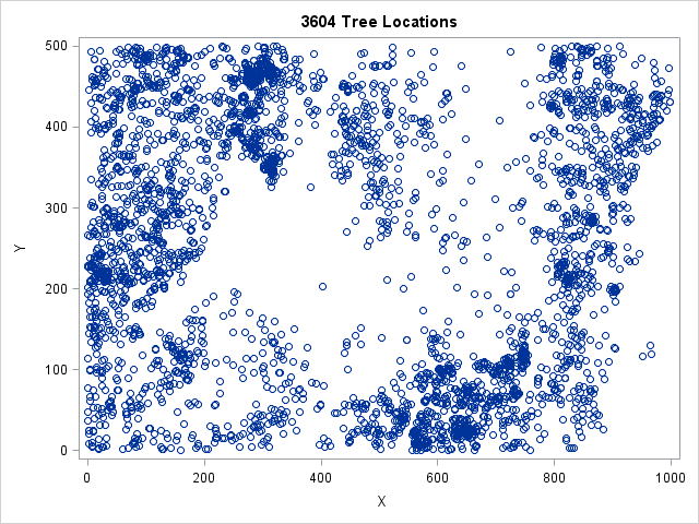
The Sashelp.Bei data contains the locations for 3,604 trees in a forest. A scatter plot of the data is shown to the left. The trees appear to be clustered in certain regions, whereas other regions contain no trees. This indicates that the trees are not uniformly distributed throughout the region.

Let's use the NearestNbr module from my previous blog post to compute the nearest neighbor distances for these tree locations. The following program saves the distances to a SAS data set named Dist_Trees. For comparison, the program also generates 3,604 random (uniformly distributed) points in the same rectangular region. The nearest neighbor distances for these simulated points are written to a data set named Dist_Unif.

proc iml;
use Sashelp.Bei where(Trees=1);
   read all var {x y} into T;
close Sashelp.Bei;
 
/* See https://blogs.sas.com/content/iml/2016/09/14/nearest-neighbors-sas.html */
start NearestNbr(idx, dist, X, k=1);
   N = nrow(X);  p = ncol(X);
   idx = j(N, k, .);   dist = j(N, k, .);
   D = distance(X);
   D[do(1, N*N, N+1)] = .;      /* set diagonal elements to missing */
   do j = 1 to k;
      dist[,j] = D[ ,><];       /* smallest distance in each row */
      idx[,j] = D[ ,>:<];       /* column of smallest distance in each row */
      if j < k then do;         /* prepare for next closest neighbors */
         ndx = sub2ndx(dimension(D), T(1:N)||idx[,j]);
         D[ndx] = .;            /* set elements to missing */
      end;      
   end;
finish;
 
run NearestNbr(nbrIdx, dist, T);
create Dist_Trees var "Dist";  append;  close; /* tree distances */
 
/* compare with uniform */
call randseed(12345);
N = nrow(T);
/* generate random uniform points in [0,1000] x [0,500] */
X = 1000*randfun(N, "uniform") || 500*randfun(N, "uniform"); 
run NearestNbr(nbrIdx, dist, X);
create Dist_Unif var "Dist";  append;  close; /* random uniform distances */
QUIT;

You can use a PROC UNIVARIATE to compare the two distributions of distances. The following DATA step merges the distances and adds an indicator variable that has the value "Uniform" or "Trees." PROC UNIVARIATE creates a graph of the empirical cumulative distribution function for each set of nearest-neighbor distances:

data All;
set Dist_Unif(in=inUnif) Dist_Trees;
if inUnif then  Group = "Uniform";
else            Group = "Trees  ";
run;
 
proc univariate data=All;
where dist<=20;   /* excludes 41 trees and 1 random observation */
   class Group;
   cdfplot dist / vscale=proportion odstitle="Compare ECDF for Uniform and Tree Data" overlay;
   ods select cdfplot;
run;

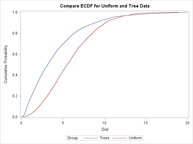
The empirical CDFs for the two data sets look quite different. For the tree data, the distribution function rises rapidly, which indicates that many observations have nearest neighbors that are very close. You can see that about 25% of trees have a nearest neighbor within about 1.5 units, and 50% have a nearest neighbor within 3.2 units.

In contrast, the empirical distribution of the uniform data rises less steeply. For the simulated observations, only 5% have a nearest neighbor within 1.5 units. Only 21% have a nearest neighbor within 3.5 units. The graph indicates clumping in the tree data: the typical tree has a neighbor that is closer than would be expected for random uniform locations.

Analysis of spatial point patterns in SAS

In SAS/STAT 13.2 and beyond you can use the new SPP procedure to perform comparisons like this automatically. The SPP procedure supports several statistical tests for "complete spatial randomness," which enable you to compare the observed distribution to the expected distribution for uniformly distributed data.

The SPP procedure supports tests that are based on nearest-neighbor distances, as well as other tests. The example in this article is essentially a visual representation of the "G function test," which you can carry out by using the following statements:

proc spp data=sashelp.bei plots=(G(unpack));
   process trees = (x, y /area=(0,0,1000,500) Event=Trees) / G;
run;

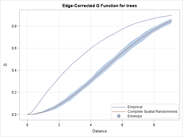
The SPP procedure creates a graph of the "edge-corrected G function." The upper curve is the empirical distribution of nearest neighbor distances for the trees, adjusted for edge effects caused by a finite domain. The lower curve shows the expected distribution for random uniform data of the same size on the same domain. The light-blue band is a 95% confidence envelope, which gives you a feeling for the variation due to random sampling. The envelope is formed by 100 simulations of random uniform data, similar to the simulation in the previous section.

The graph indicates that there is structure in the trees data beyond what you would expect from complete spatial randomness. You can use other features of PROC SPP to model the trees data. For an overview of the spatial analyses that you can perform with PROC SPP, see Mohan and Tobias (2015), "Analyzing Spatial Point Patterns Using the New SPP Procedure".

In summary, nearest-neighbor distances are useful for analyzing properties of spatial point patterns. This article compared tree data to a single instance of random uniform data. By using the SPP procedure, you can run a more complete analysis and obtain graphs and related statistics with minimal effort.