Last week Sanjay Matange wrote about a new SAS 9.4m3 option that enables you to show all categories in a graph legend, even when the data do not contain all the categories. Sanjay's example was a chart that showed medical conditions classified according to the scale "Mild," "Moderate," and "Severe." He showed how to display all these categories in a legend, even if the data set does not contain any instances of "Severe." The technique is valid for SAS 9.4m3, in which the DATTRMAP= data set supports a special column named SHOW that tells the legend the complete list of categories.

If you are running an earlier version of SAS, you can use a trick that accomplishes the same result. The trick is to create a set of all categories (in the order you want them to appear in the legend) and prepend these "fake observations" to the top of your data set. All other variables for the fake observations are set to missing values. When PROC SGPLOT reads the data for the categorical variable, it encounters all categories. However, the missing values in the other variables prevent the fake observations from appearing in the graph. (The exception is a graph that shows ONLY the categorical variable, but you can handle that case, too.)

Data that excludes a valid category

Let's create a data set that shows the problem. The SasHelp.Heart data set contains observations about patients in a medical study. The data set includes variables for the height and weight of the patient and a categorical variable called Weight_Status that has the values "Underweight," "Normal," and "Overweight." The following DATA step extracts a subset of 200 observations in which no patient is "Underweight." The call to PROC SGPLOT creates a scatter plot of the heights and weights and uses the GROUP= option to color each marker according to the Weight_Status variable.

data Heart;
set Sashelp.Heart;
where Weight >= 125;
keep Height Weight Weight_Status;
if _N_ <= 200;
run;
 
/* This scatter plot shows three problems: 
   1) The order of GROUP= variable is unspecified (default is GROUPORDER=DATA)
   2) The colors are assigned to the wrong categories
   3) The "Underweight" category is missing from the legend */
title "This scatter plot has problems!";
proc sgplot data=Heart; 
  /* attempt to assign colors for underweight=green, normal=blue, overweight=red */
  styleattrs datacontrastcolors = (lightgreen blue lightred); 
  scatter x=height y=Weight / group=Weight_Status 
                              markerattrs=(symbol=CircleFilled);
run;

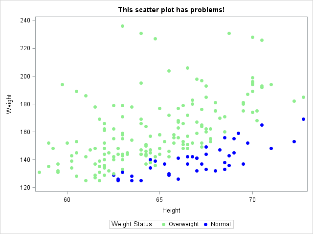
There are several problems with this scatter plot. I tried to use the STYLEATTRS statement to assign the colors green, blue, and red to the categories "Underweight," "Normal," and "Overweight," respectively. However, that effort was thwarted by the fact that the default order of the colors is determined by the order of the (two!) categories in the data set. How can I get the correct colors, and also get the legend to display the "Underweight" category?

A useful trick: Prepend fake data

The "fake data" trick is useful in many situations, not just for legends. I have used it to specify the order of a categorical variable in a graph or analysis. For example, it is useful for a PROC FREQ analysis because PROC FREQ supports an ORDER=DATA option.

The trick has three steps:

1. Create a data set that contains only one categorical variable. Specify the complete set of possible values in the order in which you want the values to be displayed.
2. Use the SET statement in the DATA step to append the real data after the fake data. The DATA step will automatically assign missing values to all unspecified variables for the fake observations. On the SET statement, use the IN= data set option to create a new indicator variable called FREQ. This new variable will have the value 0 for the fake observations and the value 1 for the real observations. (Or, if your data set already has a frequency variable, multiply the existing variable by 0 or 1.)
3. Use the newly appended data set to plot the data as usual. When you use the GROUP= option, the legends, colors, and order of categories will appear correctly because the data now contains all categories. Missing values prevent the fake observations from appearing in your plots.

The following statements illustrate the three steps for the Weight_Status variable in the Heart data set:

/* Step 1: Create a data set that contains all categories, in order */
data AllCategories;
input Weight_Status $11.;
datalines;
Underweight
Normal
Overweight
;
 
/* Step 2: Append the fake and real data. Create indicator variable. */
data Heart2;
set AllCategories         /* the fake data, which contains all categories */
    Heart(in=IsRealData); /* the original data */
Freq = IsRealData;        /* 1 for the real data; 0 for the fake data */
run;
 
/* Step 3: Use appended data set and plot as usual */
title "Include All Categories in Legend";
proc sgplot data=Heart2; 
  styleattrs datacontrastcolors = (lightgreen blue lightred);
  scatter x=height y=Weight / group= Weight_Status 
                              markerattrs=(size=9 symbol=CircleFilled);
run;

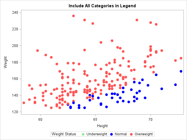
In this graph, the legend display all possible categories, and the categories appear in the correct order. The STYLEATTRS statement has correctly assigned colors to categories because you knew the order of the categories in the data set.

Graphs of the categorical variable

Adding new observations can create problems if you aren't careful. For example, suppose you use the Heart2 data set and create a bar chart of the Weight_Status variable. Unless you correct for the fake data, the bar chart will show 203 observations and display a bar for the "Underweight" category, which is not part of the original data.

The solution to this dilemma is to use a FREQ= or WEIGHT= option when you create graphs of the modified variable. The DATA step that appended the fake data also added an indicator variable, which you can use to prevent SAS procedures from displaying or analyzing the fake data, as follows:

title "Restrict to Real Data";
proc sgplot data=Heart2; 
  vbar Weight_Status /  freq=Freq;   /* do not use the fake data */
run;

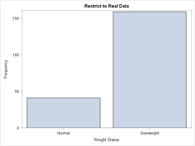
Notice that the bar chart shows only the 200 original observations. The FREQ=Freq statement uses the indicator variable (Freq) to omit the fake data.

In summary, by prepending "fake data" to your data set, you can ensure that all categories appear in legends. As a bonus, the same trick enables you to specify the order of categories in a legend. In short, prepending fake data is a useful trick to add to your SAS toolbox of techniques.