This is the last post in my recent series of articles on computing contours in SAS. Last month a SAS customer asked how to compute the contours of the bivariate normal cumulative distribution function (CDF). Answering that question in a single blog post would have resulted in a long article, therefore, I divided the task into smaller subtasks, many of which are interesting and useful on their own.

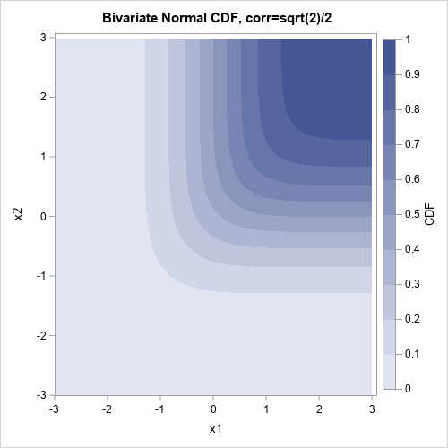
As a reminder, the adjacent image shows the contours of the bivariate normal CDF. Notice that this is not the density; it is the 2D cumulative distribution. The goal of this article is to compute a points along any specific level set (contour).

You can use the following steps to compute the contours of the bivariate normal CDF:

1. Find an initial point (x₀, y₀) that is on the contour.
2. Compute the gradient at (x₀, y₀) and use that to compute the perpendicular vector field whose trajectories are the contours.
3. Use an ODE solver to compute the trajectory/contour that passes through (x₀, y₀).

1. Find an initial point on the contour

Let F(x,y;ρ) denote the cumulative distribution function for the bivariate standard normal distribution with correlation ρ. In SAS, you can use the PROBBNRM function to evaluate the bivariate normal distribution.

It is evident from the previous graph that every contour of F intersects the diagonal line y = x. You can use this fact to find an initial point on a contour: Given a level, c, find the value of x such that F(x,x;ρ) = c. Equivalently, you can find a root (zero) of the function F(x,x;ρ) - c.

The following SAS/IML statements use a root-finding algorithm (the FROOT function in the SAS/IML language) to find a value of x such that (x,x) is on a specified contour. If you are running a version of prior to SAS/IML 12.1, use the bisection module instead of the FROOT function.

proc iml;
g_rho = 0.5;       /* global variable for the bivariate correlation */
g_level = 0.1;     /* global variable for the contour level */
 
/* Restrict PROBBNRM function to line y=x and subtract the given level, g_level. 
   The (unique) zero of this function is a point on the contour F(x,y;g_rho)=c */
start DiagCDF(x) global(g_level, g_rho);
   return( probbnrm(x, x, g_rho) - g_level );
finish;
 
/* If c is in (0, 1), find the point (x,x) such that PROBBNRM(x,x,rho)=c */
start ContourPt(range);
   z = froot("DiagCDF", range);  /* for example, search for x in [-5,5] */
   return( z||z );
finish;

Remark: A plot of the function F(x,x;ρ) looks very much like a normal CDF function. Does anyone know whether this is true? Can you find a value of μ and σ such that Φ(x; μ, σ) = F(x,x; ρ)? If so, you don't need to use the FROOT function. You could instead use the QUANTILE function, which would be faster and more accurate.

2. Compute the perpendicular to the gradient

The next step is to define a function that returns a vector that is perpendicular to ∇F(x,y), the gradient vector at an arbitrary point (x,y). Obviously, if u is perpendicular to ∇F, then so is –u. I've previously shown how to compute the gradient of the bivariate normal cumulative distribution. The following SAS/IML program defines the gradient of F, and two vector fields that are perpendicular to the gradient field. The functions for the perpendicular fields have a strange signature (they take t as an argument, even though they are not time-varying vector fields) because they will be called by the ODE function in Step 3.

start GradCDF(x) global(g_rho);
   dfdx = pdf("Normal", x[1]) * cdf("Normal", x[2], g_rho*x[1], sqrt(1-g_rho##2));
   dfdy = pdf("Normal", x[2]) * cdf("Normal", x[1], g_rho*x[2], sqrt(1-g_rho##2));
   return( dfdx // dfdy );
finish;
 
start PerpGrad(t, x);
   g = GradCDF(x);
   return( (-g[2] // g[1]) / norm(g) );
finish;
 
start NegPerpGrad(t, x);
   return( -PerpGrad(t,x) );
finish;

3. Compute the contour

This step computes the contour that passes through the point that was found in Step 1. The method uses the fact that the contour is the trajectory of the perpendicular vector field(s) that are defined in Step 2. Two trajectories are computed: one for the perpendicular vector field, and the other for the negative of that field. This is equivalent to integrating forward in time, followed by integrating backwards in time. The two trajectories are concatenated together into a single contour.

The following statements compute the level sets for c ∈ {0.1, 0.2,..., 0.9}. The trajectories are all saved to a SAS data set named CDFContour.

h = {1.e-8 1 1e-3};                      /* min, max, and initial time steps */
time = do(0,5,0.1);
p = .; x=.; y=.;                         /* specify that vars are numeric */
create CDFContour var {"p" "x" "y"};     /* open data set for writing */
 
probs = do(0.1, 0.9, 0.1);
do i = 1 to ncol(probs);
   g_level = probs[i];
   x0 = ContourPt({-5 5});                /* Find one point on the contour */
   call ode(s1,"PerpGrad",x0`,time,h);    /* Trace contour in one direction */
   call ode(s2,"NegPerpGrad",x0`,time,h); /* Trace contour in other direction */
   soln = s2[,ncol(s2):1] || x0` || s1;
   x = soln[1,];  y = soln[2,]; p = j(1,ncol(x),probs[i]);   
   append;                                /* write trajectory */
end;
close CDFContour;
quit;

title "Contours of Bivariate Normal Cumulative Distribution";
proc sgplot data=CDFContour aspect=1;
   where (x<=3 & y<=3);
   label p = "P(X<x & Y<y)";
   series x=x y=y / group=p curvelabel curvelabelpos=max;
   xaxis grid min=-2 max=3;
   yaxis grid min=-2 max=3;
run;

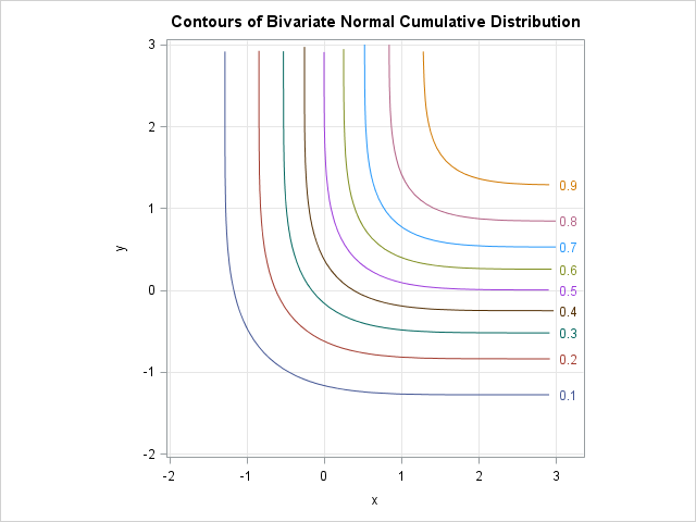
In conclusion, you can work out the formulas necessary to compute any specified contour for the bivariate cumulative normal distribution. The contours in the previous graph, which were computed by using the ODE function in SAS/IML software, are similar to the contours shown at the beginning of this article, which were computed (automatically) by using the ODS statistical graphics in SAS. If you only need to view a contour plot, use ODS statistical graphics to draw the contour plot. However, if you need to compute points along a specific contour, you can use the techniques that are presented in this article.