Like many other computer packages, SAS can produce a contour plot that shows the level sets of a function of two variables. For example, I've previously written blogs that use contour plots to visualize the bivariate normal density function and to visualize the cumulative normal distribution function.
However, sometimes you don't just want to see a picture of the contours, you actually want to compute a sequence of points along a specific contour. There are several algorithms for computing contours, but this article describes a technique known as a continuation method, or a predictor-corrector algorithm.
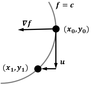
The continuation method is illustrated by the graphic to the left. Start with an initial point (x0, y0) that is on the contour. The gradient at (x0, y0) is perpendicular to the contour at that point, so you can compute the tangent to the contour. You can then take a small step in the tangent direction (the predictor step). Usually, the step takes you off the contour, so you need to re-acquire the contour (the corrector step). You now have a new point on the contour, so you can repeat the process.
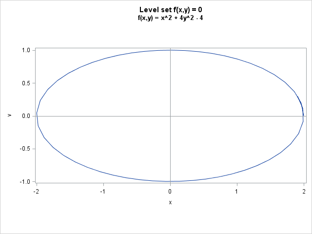
Because the algorithm uses gradient information, it is often possible to form the tangent vector analytically. To give a simple example, suppose that you are interested in tracing the level set {(x,y} | f(x,y)=0} where f is the quadratic function, f(x,y) = x2 + 4y2 - 4. The gradient vector is (2x, 8y). For this function, the contour is an ellipse that passes through the point (2, 0).
The following SAS/IML program defines the quadratic function, the gradient of the function, and the vector field that is perpendicular to the gradient field. The perpendicular field is normalized so that each vector has length one. This means that the perpendicular field is undefined at the critical points of f, where the gradient vanishes.
proc iml; /* we want contours for this function */ start Func(x); f = x[,1]##2 + 4#x[,2]##2 - 4; return( f ); finish; /* gradient of function (df/dx, df/dy) */ start Grad(x); dfdx = 2#x[1]; dfdy = 8#x[2]; return( dfdx // dfdy ); finish; /* normalized vector field that is perpendicular to the gradient field (-df/dy, df/dx) / norm(gradient) */ start PerpGrad(t, x); g = Grad(x); return( (-g[2] // g[1]) / norm(g) ); finish; |
Now the interesting fact about the predictor-corrector algorithm is this: the contour-tracing algorithm described above is the same as the predictor-corrector algorithm that is used to solve differential equations! Let G be a vector field that is perpendicular to the gradient field. Then the contour that passes through (x0, y0) is exactly the same as the trajectory of G with initial condition (x0, y0). (For contours that are not closed curves, you also need to integrate "backwards" by using the vector field -G, which is also perpendicular to the gradient field.)
By a fortunate coincidence, I blogged last week about how to solve differential equations in SAS. Although I didn't say it at the time, the phase portraits for the simple harmonic oscillator and the pendulum are plots that show contours. The trajectories are level sets of the "total energy function," which is the sum of the potential and kinetic energies for those mechanical systems.
The following call to the ODE subroutine computes a contour for the quadratic function. It is the level set for 0, which passes through the point (2, 0).
/* use ODE to integrate vector field perpendicular to gradient */
x0 = {2, 0};           /* initial values */
t = do(0, 10, 0.2);    /* compute solution at these time pts */
h = {1.e-6 1 1e-3};    /* min, max, and initial step size */
call ode(soln, "PerpGrad", x0, t, h);

/* write trajectory to a SAS data set */
x = t` || (x0` // soln`);
create Contour from x[c={"t" "x" "v"}]; append from x; close Contour;
quit;

/* plot the contour */
title "Level set f(x,y) = 0";
title2 "f(x,y) = x^2 + 4y^2 - 4";
proc sgplot data=Contour aspect=0.5; /* ASPECT= is 9.4 option */
   series x=x y=v;
   refline 0 / axis=x;
   refline 0 / axis=y;
run; |
The take-away message is this: you can compute (nonsingular) contours by integrating a vector field that is perpendicular to the gradient field. The same predictor-corrector algorithm that solves differential equations can be used to trace contours.

1 Comment
Pingback: Compute contours of the bivariate normal CDF - The DO Loop