It is easy to simulate data that is uniformly distributed in the unit cube for any dimension. However, it is less obvious how to generate data in the unit simplex.
The simplex is the set of points (x1,x2,...,xd) such that Σi xi = 1 and 0 ≤ xi ≤ 1 for i = 1,2,...,d. Because the elements sum to 1, a uniform distribution on the unit simplex can be used for many statistical tasks, such as drawing a probability vector with d elements.
The simplest algorithm I know is Algorithm 3.23 in Kroese, Taimre, and Botev, (2011, p. 73), Handbook of Monte Carlo Methods, which generates N points from the exponential distribution and uses the fact that the interval between consecutive points in an exponential distribution are uniformly distributed. You can implement this algorithm by using the SAS DATA step or by using the following SAS/IML function:
proc iml; /* generate points in standard simplex by using Algorithm 3.23 in Kroese, Taimre, and Botev, (2011, p. 73) */ start RandUniSimplex(N, d); x = j(N, d); /* allocate matrix */ call randgen(x, "Exponential"); /* fill with x ~ Exp */ return( x / x[,+] ); /* set row sums to 1 */ finish; |
Recall that the expression x[,+] is a subscript reduction operator that returns the sum of the elements in each row of x.
To test the function, simulate 1,000 observations from the uniform distribution on the unit simplex in three dimensions. The data should be uniformly distributed on a planar triangle with vertices (1,0,0), (0,1,0) and (0,0,1). To visualize the simulated data, you can write the data in the matrix to a SAS data set and use the SGPLOT procedure to display a scatter plot of the first two coordinates:
call randseed(1);
x = RandUniSimplex(1000, 3);  /* generate obs in 3D simplex */

create Simplex from x[c=("x1":"x3")];
append from x;
close Simplex;

proc sgplot data=Simplex;
   title "Uniform Distribution in the Unit Simplex";
   scatter x=x1 y=x2;
run; |
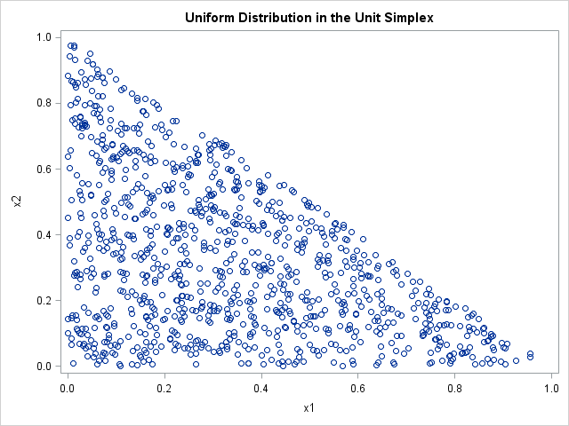
The graph shows that first two variables are uniformly distributed in the two-dimensional unit simplex. The third coordinate is not shown because it is trivially derived from the first two: x3 = 1 – x1 – x2.
