I was at the Wikipedia site the other day, looking up properties of the Chi-square distribution. I noticed that the formula for the median of the chi-square distribution with d degrees of freedom is given as ≈ d(1-2/(9d))3. However, there is no mention of how well this formula approximates the true value of the median, nor is there a reference. (Please post a comment if you know where this formula is derived.)
The formula is a model for the value of the median. As such, it contains modeling error. By using the SAS/IML language or the SAS DATA step, you can compare this model to a direct numerical computation of the median.
As John D. Cook discussed, the error introduced by a model (the formula) can be orders of magnitude greater than the approximation error from a finite precision numerical computation. Let's compare the formula to a numerical computation of the median for a range of degrees of freedom. The median is the 0.5 quantile, so you can use the QUANTILE function to compute the "true" median. ("True" is in quotes because the computation is itself an approximation, but the approximation error should be small.) The following program computes the difference between the median values of the chi-square distribution as returned by the QUANTILE function and as computed by using the Wikipedia formula:
proc iml;
d = do(0.1,0.3,0.005) || do(0.4, 6, 0.1); /* range of degree of freedom */
q = quantile("chisquare", 0.5, d); /* "true" computation */
formula = d#(1-2/(9*d))##3;
diff = q-formula; |
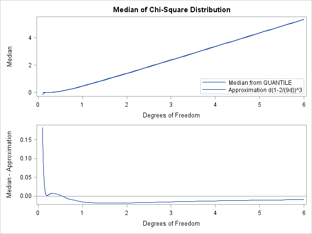
I've plotted the results. In the top graph, the "true" and approximate medians look identical except when the degree of freedom, d, is very small (for example, d < 0.125). However, there is a general rule to follow when you are trying to understand how two similar quantities differ: Do not plot the quantities themselves (the top graph), but rather plot the difference between the quantities (the bottom graph).
When you plot the difference, you get a better sense for the approximation. The formula appears to be biased for d > 1, since the formula is always less than the true median.
Is the formula of any value? Yes. It is a model, and models are good for showing us the big picture. The formula shows that the median increases roughly linearly with the degree of freedom. The formula is also useful for understanding the asymptotic value of the median: For a large degree of freedom, d, the formula indicates that the median is approximately d - 2/3. (I've used the approximation (1-x)3 ≈ (1-3x) for small x.)
Incidentally, the formula is a Laurent polynomial, which means that it includes both positive and negative powers of d. Laurent polynomials can be useful in numerical analysis, but you don't see them as often as their better-known cousin, the Taylor polynomial. A Laurent polynomial can capture the behavior of a function near zero (where Taylor polynomials also succeed) and far from zero (where Taylor polynomials often fail).

12 Comments
Dear Rick Wicklin,
Thanks for posting useful info about SAS/IML on this weblog and sorry that this comment in not related to this post.
I have been looking for a command in SAS/IML which finds the location of the matched values in two different vectors.
I came across this website: http://stackoverflow.com/questions/4952548/value-matching-in-sas-iml where the same question was asked and you suggested using XSECT function to find the intersection of the two sets. However, XSECT function gives the common elements between two sets rather that giving the location of those elements.
For example, in the following code:
proc iml;
x={10 11 12 13 12 13 14 15};
v={12 13};
z=xsect(x,v);
print z;
quit;
the SAS results are: Z= {12 13}, but I’m looking for a vector like {3 4 5 6} which is the location of common elements of vector V in vector X.
Would you please provide me with the appropriate function in SAS/IML?
Thank you very much.
You can ask questions related to SAS/IML programming at the SAS/IML Discussion forum:
http://communities.sas.com/community/sas_iml_and_sas_iml_studio
Dear Rick Wicklin,
You ask if anybody knows where the approximation ≈ d(1-2/(9d))3 comes from. I looked up chi-square in the bible of functions, Abramowitz and Stegun, and stumbled upon formula 26.4.14, which states that if d>30, then the transformed variable x_2 = ( (x/d)^(1/3) –(1-2/9d) ) / \sqrt(2/9d) is standard normal distributed. And when that’s the case, the median Is X_2=0 and hence the above approximation.
This approximation is a statement about the entire distribution; however from your graphs it seems safe to apply the median approximation for even lower degrees of freedom.
(Where Abramowitz and Stegun have their result from I have no idea.)
Interesting. Thanks!
While trying to find your formula, I stumbled upon 26.2.49, which approximates the inverse CDF (quantile function) of an ARBITRARY distribution in terms of Hermite polynomials! It's amazing what's in that tome.
Dear Rick,
About the approximation for the median of a chi-square distribution that you recommend, (1-x)^3, I just wanted to ask you:
1. For which values of x does it apply? I guess that just for x<1, but please let me know if I'm wrong.
2. Is there a published paper (yours of from someone else) that stands after such an approximation?. This is because I would like to use such a formula in a document that I'm working in, but I would like to have a formal reference about it.
Thanks in advance for your kind repply,
I think you misread the article. I did not claim that the median is approximately (1-x)^3. What I said is that the median of a chi-sq(d) distribution is approximately d(1-2/(9d))^3 when d > 0.125. I also said that the median is approximately d - 2/3 for sufficiently large values of d. "Sufficiently large" means that d >> 2/9 (which is read "much much greater than 2/9"). Empirically, d > 1 is probably good enough.
Regarding citation, you can cite this blog as
Wicklin, Rick (2011) "On the median of the chi-square distribution," published in The DO Loop blog, 09NOV2011.
URL: https://blogs.sas.com/content/iml/2011/11/09/on-the-median-of-the-chi-square-distribution.html
Sir this have any proof then reply me .Yesterday I had learned that this distribution does not have median
It has a median. What you probably heard is that there is no simple formula for the median in terms of elementary functions.
I got here while trying to find a source for this myself. I didn't find the original source exactly as stated, but found what it comes from, and ordered a 1970 stat book that seems to have a section on the history of such things. It follows trivially from the approximate normalization formula given in Abdel-Aty, S. H. "Approximate Formulae for the Percentage Points and the Probability Integral of the Non-central χ 2 Distribution." Biometrika 41.3/4 (1954): 538-540.
If you want a much better approximation (for integer numbers of degrees of freedom d, down to 1, below which the chi-square distribution is not defined), try this: (d + 2*log(2) - 2/3 + 0.115668/(d + 0.1598) ) / 4^(1/d). See if you can figure out where that comes from.
Actually, it goes back to 1931. Abdel-Aty references for that central case (though he misspells Hilferty as Hilfertz):
Wilson, Edwin B., and Margaret M. Hilferty. "The distribution of chi-square." Proceedings of the National Academy of Sciences 17.12 (1931): 684.
And so does Wikipedia; see the Wilson-Hilferty transformation (same as was pointed out in Abramowitz and Stegun), even in the 2011 version you started with: the Wilson-Hilferty transformation. Too bad the connection wasn't made there. I'll fix it.
Can you explain the relation of the median and variance of a Chi-Squared distribution.
The variance is 2*d, so the ratio of (Variance/Median) is approximately 2/(1-2/(9*d))^3 when d > 0.125. If d is sufficiently large (such as d > 1), then the ratio is approximately (2*d)/(d - 2/3), which approaches 2 for very large d.