I was contacted by SAS Technical Support regarding a customer who was trying to use SAS/IML to compute quantiles of the folded normal distribution. I had heard of the distribution, but it is not built into SAS and I had never worked with it. Nevertheless, I set out to understand the distribution and figured out how to compute it's various important properties.
As I mentioned last week, there are four essential functions that you need when you are working with a statistical distribution. You need to know how to generate random values, how to compute the PDF, how to compute the CDF, and how to compute quantiles. In this article, I describe how to compute each of the four essential quantities for the folded normal distribution. In this way, you can see how to use SAS/IML to define these functions for distributions that are not explicitly built into SAS.
Random Values of the Folded Normal Distribution
The Wikipedia article on the folded normal distribution states, "Given a normally distributed random variable X with mean μ and variance σ2, the random variable Y = |X| has a folded normal distribution." By using this definition, it is easy to write down the function that generates a random sample:
proc iml; start RandFolded(x, mu, sigma); call randgen(x, "Normal", mu, sigma); x = abs(x); finish; /* test: generate 1,000 random values from the folded normal */ call randseed(12345); mu = 1; sigma = 1; /* parameters of the distribution */ y = j(1000, 1); call RandFolded(y, mu, sigma); |
A histogram of the random sample is shown in the following plot. The histogram is overlaid with a curve that shows the PDF for the folded normal distribution, which is computed in the next section.
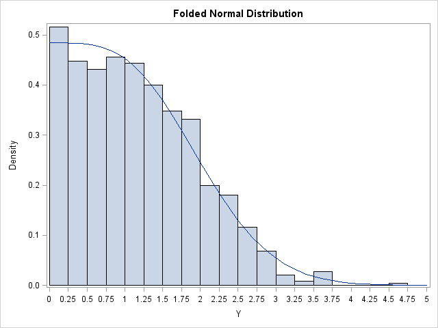
The PDF for the Folded Normal Distribution
The folded normal distribution is "folded" in the sense that the density for the normal distribution is "folded over" across the x=0 line. That means that the density at some point x>0 is given by the sum of the density of the normal distribution at x and the density of the normal distribution at -x. This is coded as follows:
start PDFFolded(x, mu, sigma);
   return( pdf("Normal",  x, mu, sigma) +
           pdf("Normal", -x, mu, sigma) );
finish;

/* test: generate PDF for a sequence of points */
x=T( do(0,4,0.1) );
pdf = PDFFolded(x, mu, sigma); |
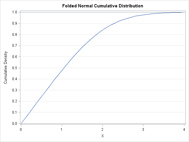
The CDF for the Folded Normal Distribution
You can express the CDF for the folded normal distribution in terms of the CDF for the normal distribution. When you integrate the PDF of the folded normal distribution, a negative sign appears during a change of variables (see the Wikipedia article), and you get the following CDF:
start CDFFolded(x, mu, sigma);
   return( cdf("Normal",  x, mu, sigma) -
           cdf("Normal", -x, mu, sigma) );
finish;

/* test: generate CDF for a sequence of points */
cdf = CDFFolded(x, mu, sigma); |
Quantiles for the Folded Normal Distribution
So far, everything has been easy. For the folded normal distribution, it is possible to express the PDF, the CDF, and the "RAND" functions by using the corresponding functions for the normal distribution. Unfortunately, I don't think it is possible to compute quantiles of the folded normal in terms of quantiles of the normal distribution.
However, all is not lost. The CDF is continuous and monotone increasing, so it is easy to compute quantiles by using a root-finding technique. Given a probability, p, the pth quantile is simply the value q such that CDF(q)=p, or, equivalently, for which CDF(q)-p=0.
I previously wrote about using bisection to compute the roots of a univariate function, so I'll reuse the Bisection module in that article. So that I don't have to modify the Bisection module, I'll give the name "FUNC" to the function whose zeros I want to compute, which is FUNC(x) = CDF(x)-p. The root of the FUNC module is the pth quantile of the folded normal distribution:
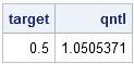
/* load or define bisection module here */ /* a quantile is a zero of the following function */ start func(x) global(mu, sigma, target); return( CDFFolded(x, mu, sigma)-target ); finish; /* test: compute the median (0.5 quantile) */ target = 0.5; qntl = Bisection(0, 4); /* search on interval [0,4] */ print target qntl; |
Fit a folded normal distribution to data
You can use SAS/IML to fit a folded normal distribution to data by using the method of maximum likelihood estimation. An example is shown in the documentation for PROC UNIVARIATE.
Conclusions
The PDF, CDF, QUANTILE, and RAND functions in SAS support the distributions that arise often in practice. This article shows how you can use these distributions as building blocks to define new distributions, such as the folded normal distribution.

2 Comments
Pingback: Compute the quantiles of any distribution - The DO Loop
Pingback: Levy flight and vectorizing a simulation in SAS - The DO Loop