At the SAS/IML Support Community, a SAS/IML programmer recently asked how to find "the root of a complicated equation."
That's a huge question, and many papers and books have been written on the topic of root-finding, also known as finding the zeros of a function.
Everyone has favorite techniques for root-finding. My approach is to use simple techniques first, and only proceed to more complicated algorithms if the simple techniques fail or are too slow. The first technique that I try depends on the function:
- For a polynomial function of one variable, use the POLYROOT function in SAS/IML software.
- For a non-polynomial function of one variable:
- First bracket the root. This means finding an interval [a,b] so that f(a) and f(b) have opposite signs.
- Use bisection or Brent's method to solve for the root in the interval.
- For a function of several variables, try Newton's method, which is simple to program and converges quickly to a root when the algorithm starts near a root.
The following sections implement two univariate techniques in SAS/IML software. On Friday, I'll discuss Newton's method.
Roots of Polynomials
In the SAS/IML language, the POLYROOT function solves for the roots of a univariate polynomial with real coefficients. The input to the POLYROOT function is a vector that contains the coefficients of the polynomial, ordered by decreasing powers of the polynomial terms. This might be the opposite of what you expect. In the following statements, p[1] is the coefficient of the cubic term, and p[4] is the constant term:
proc iml;
/** x##3 - 2 x##2 -4 x + 3 **/
p = {1, -2, -4, 3};
roots = polyroot(p);
print roots; |
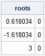
The third-degree polynomial in this example has three real roots: -1.618, 0.618, and 3. The POLYROOT function returns a matrix with two columns. Each row is the real and imaginary parts of the roots of the polynomial. If you are interested only in the real roots, restrict your attention to the roots that contain a zero in the second column.
Roots of an Arbitrary Univariate Function
This section shows how to compute the real roots of an arbitrary function of one variable by using the bisection method. The bisection method is probably the simplest root-finding method imaginable. After bracketing the root, you subdivide the bracketing interval and determine which half contains the root. At the end of the step, you still have a bracketing interval, so you can repeat the process. The advantages of the bisection algorithm are:
- It is trivial to program.
- It essentially always works.
- It does not require any information about the derivative of the function.
The disadvantage is that the method converges linearly to a root, whereas most other root-finding algorithms converge super-linearly. An alternative to the bisection algorithm is Brent's method. Although harder to program, Brent's method is also very robust and does not require derivative information. For an alternative method that requires derivatives, see the following post on Newton's Method.
The first step is to graph the function in order to get a feel for its behavior and the approximate locations of its roots. From the graph, you can often visually bracket a root. You can then use a bracketing algorithm to approximate the root. In the following statements, I use the LinePlot class in IMLPlus to graph the function in SAS/IML Studio. You can also use PROC SGPLOT if you are not using SAS/IML Studio.
/** define function and plot **/
start Func(x);
   return( exp(-x##2) - x##3 + 5#x +1 );
finish;
x = do(-5,5,0.1);
LinePlot.Create("roots", x, Func(x)); /** IMLPlus **/ |
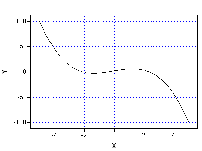
There are three roots to this function. The following statements use the bisection method to approximate the root on the interval [2,3].
/** Bisection: find root on bracketing interval [a,b].
    If x0 is the true root, find c such that
    either |x0-c| < dx or |f(c)| < dy.
    You could pass dx and dx as parameters. **/
start bisection(a, b);
dx = 1e-6; dy = 1e-4;
do i = 1 to 100; /** max iterations **/
   c = (a+b)/2;
   if abs(func(c)) < dy | (b-a)/2 < dx then
      return(c);
   if func(a)#func(c) > 0 then a = c;
   else b = c;
end;
return (.); /** no convergence **/
finish;

z = bisection(2, 3);
print z; |

The algorithm stops if it requires more than 100 iterations, although you can actually determine the maximum number of iterations because the interval [a,b] is cut in half during each step. The algorithm also stops if FUNC(c) is small (less than dy in absolute value), or if the bracketing interval is small (less than dx). Some people prefer to stop when BOTH of those criteria are satisfied, in which case the DO loop becomes necessary to prevent infinite loops when evaluating functions that are extremely flat or steep near the root.

7 Comments
Rick:
I think the code you posted for the bisection algorithm contained a typo (missing something):
This statement is syntactically incorrect because it is missing an operator:
if abs(Func(c)) < dy | (b-a)/2 0 then a = c;
Thanks. SAS has changed to a new blog platform and there are a few bugs that we need to work out concerning posting code. Please read the code carefully over the next few weeks spot problems like you reported.
Pingback: Using Newton’s Method to Find the Zero of a Function - The DO Loop
Pingback: Evaluate polynomials efficiently by using Horner’s scheme - The DO Loop
Pingback: Implement the folded normal distribution in SAS - The DO Loop
What if i want to calculate the root of a function, but it is related to another variable, say y, y is a vector? I need x is a vector too.
start Func(x);
return( exp(-x##2) - x##3 + 5#x +y );
finish;
Depending on the formulation of the problem, roots of vector-valued functions can be found by using Newton's method or tools such as linear programming or genetic algorithms. In some situtations, you can productively find minima of ||f|| by using nonlinear optimization methods.