I've previously discussed how to find the root of a univariate function. This article describes how to find the root (zero) of a function of several variables by using Newton's method.
There have been many papers, books, and dissertations written on the topic of root-finding, so why am I blogging about a 17th-century algorithm? Newton's method is an important tool in my numerical toolbox because of three features:
- It is relatively easy to program.
- It usually converges quickly (in fact, quadratically) to a root, once it gets close.
- It works in arbitrary dimensions.
Its biggest disadvantages are:
- It requires a derivative function.
- It might not converge, or might converge to a different root than you intended.
Requiring a derivative is both an advantage and a disadvantage. It is the derivative that makes Newton's method so effective. However, it can be a tedious task to type in the derivative matrix for complicated functions. Or you might want the root of a function that does not have a closed-form analytical expression. (Perhaps it involves a simulation.) In that case, obtaining a derivative expression can be difficult and computationally expensive.
Fortunately, the advantages of Newton's method usually outweigh the disadvantages. A hidden advantage to Newton's method is that it serves as a basis for more sophisticated methods, which means that understanding Newton's method is a necessary first step towards mastering other multivariate root-finding techniques.
An Example of Newton's Method
You can implement Newton's method for multivariate functions by using the SAS/IML language. The SAS/IML documentation contains an example of Newton's method, but I don't like the coding style of the program because it uses global variables. I prefer modules that are self-contained functions with arguments and local symbol tables so that I can use them as components in other programs without worrying about side-effects.
Still, the example is pretty good, so I will use the main ideas but re-code the implementation.
The example function is a function of two variables that returns two components: f(x1, x2) = (f1(x1,x2), f2(x1,x2)), where f1(x1,x2) = x1+x2-x1*x2+2, and f2(x1,x2)= x1*exp(-x2)-1. The following statements define the function in the SAS/IML language:
proc iml; /** find roots of this function **/ start Func(x); x1 = x[1]; x2 = x[2]; f1 = x1 + x2 - x1 * x2 + 2; f2 = x1 * exp(-x2) - 1; return( f1 // f2 ); finish Func; |
Because the graph of this function is in four-dimensional space, you can't directly plot the graph of the function. However, you can visualize the locations of the zero(s) by plotting the magnitude (norm) of the function. In the following graph, I use the contour plot in SAS/IML Studio to graph the quantity || f || = sqrt(f12 + f22) on a uniform grid of (x1, x2) values.
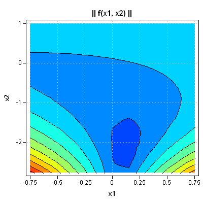
The minimum value of the function is somewhere in the dark blue region. Therefore, a good initial point to use for Newton's method is (0, -2). (The example in the SAS/IML documentation uses an initial guess of (0.1, -2), which is even closer to the root.)
Newton's Method in SAS
In order to use Newton's method, you need to write a function that computes the Jacobian matrix at an arbitrary location. The Jacobian matrix is the matrix of partial derivatives, so it is a 2 x 2 matrix for this example. The following statements define the function Deriv, which computes the Jacobian matrix.
/** derivatives of the function **/
start Deriv(x);
   x1 = x[1]; x2 = x[2];
   df1dx1 = 1-x2;
   df1dx2 = 1-x1;
   df2dx1 = exp(-x2);
   df2dx2 = -x1 * exp(-x2);
   J = (df1dx1 || df1dx2 ) //
       (df2dx1 || df2dx2 );
   return( J );
finish Deriv; |
The Newton module implements Newton's method and calls the Func and Deriv functions for each Newton step.
/** Newton's method to find roots of a function.
    You must supply the FUNC and DERIV functions
    that compute the function and the Jacobian matrix.
    Input: x0 is the starting guess
           optn[1] = max number of iterations
           optn[2] = convergence criterion for || f ||
    Output: x contains the approximation to the root **/
start Newton(x, x0, optn);
   maxIter = optn[1]; converge = optn[2];
   x = x0;
   f = Func(x);
   do iter = 1 to maxIter while(max(abs(f)) > converge);
      J = Deriv(x);
      delta = -solve(J, f); /** correction vector **/
      x = x + delta;        /** new approximation **/
      f = Func(x);
   end;
   /** return missing if no convergence **/
   if iter > maxIter then x = j(nrow(x0),ncol(x0),.);
finish Newton; |
This version of Newton's method is based on the SAS/IML documentation, but it is not the only version possible. For example, the convergence criterion for this version is that max(abs(f)) is small. This quantity is the L∞ norm. You might prefer to use the usual Euclidean norm, which is computed as sqrt(ssq(f)).
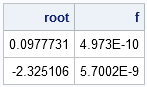
The following statements call the Newton subroutine and print the zero of the function. The function evaluated at the root is also printed, in order to verify that the function is, indeed, nearly zero.
x0 = {0, -2};     /** initial guess **/
optn = { 15,      /** maximum iterations **/
         1E-6 };  /** convergence criterion **/
run Newton(root, x0, optn);
f = Func(root);
print root f; |
In closing, I'll mention that Newton's method requires that you compute the Jacobian matrix at each iteration, which might be computationally expensive. Consequently, there are variations of Newton's method (such as Broyden's method) that compute the Jacobian fewer times, but update the Jacobian at each iteration by using less expensive numerical techniques.

4 Comments
Pingback: Using the MOD function as a debugging tool - The DO Loop
Pingback: A simple way to find the root of a function of one variable - The DO Loop
Pingback: How to choose parameters so that a distribution has a specified mean and variance - The DO Loop
Pingback: The sensitivity of Newton's method to an initial guess - The DO Loop