It has been a long time since I thought about how to create an ROC curve "by hand," so I decided to do some research. This article describes how to construct an empirical ROC curve and includes a SAS/IML module that implements the algorithm. This is the same curve obtained by Charlie's macro and by the OUTROC= option in the MODEL statement of the LOGISTIC procedure.
The intent of this article is to describe the algorithm for computing an ROC curve, not to offer a replacement for the ROC analysis in the LOGISTIC procedure. For serious data analysis, use the LOGISTIC procedure.
Basic Ideas of ROC Curves
To remind myself of the details of ROC curves, I referenced the excellent book ROC Curves for Continuous Data by W. Krzanowski and D. Hand. The notation and ideas in this article are taken from their introduction (p. 2–12) and from an example on p. 41–44.
Suppose each observation in the data is one of two groups, such as diseased and healthy. Call one of the groups P (for "positive") and the other N (for "negative"). It is useful to use the data to build a statistical model. The purpose of the model is to classify future observations into either the P or the N group by using a "score" that is obtained from explanatory variables, such as the results of laboratory tests. (For a more whimsical example, you can predict whether a person is female by knowing how many shoes the person owns.) When the score is large (greater than some threshold, t), you classify the observation into class P; when the score is small (at or below the threshold), you classify the observation into class N.
No matter how you choose the threshold, t, you are going to misclassify some subjects (unless the data are completely separable). Suppose your male/female classification rule is "predict that someone is female if the person owns more than 15 pairs of shoes." For this rule, t = 15. With such a rule, you will misclassify any males who own more than 15 pairs of shoes. These individuals are false positives: the rule puts them into class P (female), but they don't belong there. However, you correctly classify females who own more than 15 pairs of shoes. These individuals are true positives : the rule puts them into class P, and that's where they belong. (False positives and false negatives are also important in criminal trials, such as the Casey Anthony case.)
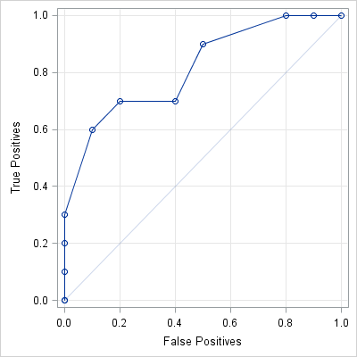
The ROC curve is a diagnostic tool that plots the proportion of true positives against the proportion of false positives for all possible values of the threshold parameter.
The Basic Ideas of Computing ROC Curves
Krzanowski and Hand (p. 41–44) compute an empirical ROC curve for the following data. For each observation, we know whether it belongs to group N or group P. The following SAS/IML statements define the data vector, x, and construct an indicator variable, y, which has the value 0 if an observation is in N, and the value 1 if an observation is in P:proc iml; /** x and y are column vectors. y contains {0,1} **/ N = {0.3,0.4,0.5,0.5,0.5,0.6,0.7,0.7,0.8,0.9}; P = {0.5,0.6,0.6,0.8,0.9,0.9,0.9,1.0,1.2,1.4}; x = N // P; y = repeat(0, nrow(N)) // repeat(1, nrow(P)); |
Krzanowski and Hand describe how to construct an empirical ROC curve for these data. For a given value of the threshold, t, the empirical classification rule predicts that an observation belongs to P if it is greater than t. The empirical true positive rate, tp, is the number of values greater t divided by 10, which is the total number of positives in the data. Similarly, the empirical false positive rate, fp, is the number values less than t divided by 10, which is the total number of negatives in the data.
To construct the ROC curve, they first set the threshold, t, to be a large value. Then (p. 43):
Consider progressively lowering the value of t. For any value greater than or equal to 1.4, all 20 observations are allocated to group N, so no P individuals are allocated to P (hence tp = 0.0) and all the N individuals are allocated to N (hence fp = 0.0). On crossing 1.4 and moving t down to 1.2, one individual (the last) in group P is now allocated to N (hence tp = 0.1) while all the N individuals are still allocated to N (hence fp = 0.0 again). Continuing in this fashion generates [the ROC curve].
The following SAS/IML module implements the algorithm for the construction of an empirical ROC curve. The input is a vector x that contains the data and a vector y that indicates whether each value belongs to P or N. Instead of counting the number of false positives, it is convenient to compute the number of true negatives (tn), and then use the identity fp = 1 – tn at the end of the module.
start ROC(x, y); /** create cutpoints (assume no missing values) **/ u = unique(x); cutpts = (u[1]-1) || u; nc = ncol(cutpts); TP = j(nc,1,.); TN = j(nc,1,.); /** allocate **/ /** count how many obs greater than and less than each cutpoint for Y=0 and Y=1 **/ x0 = x[loc(y=0)]; Num0 = nrow(x0); /** num in N **/ x1 = x[loc(y=1)]; Num1 = nrow(x1); /** num in P **/ do i = 1 to nc; /** proportions for each cutpoint **/ TN[i] = sum( x0 <= cutpts[i] ) / Num0; TP[i] = sum( x1 > cutpts[i] ) / Num1; end; /** return false pos (=1-TN) and true pos rates (1 - specificity) || sensitivity **/ return((1-TN) || TP); finish; |
The ROC module uses the UNIQUE function to find the cutpoints of the data. (These are the threshold values for which the number of true/false positives changes.) The module counts the number of elements in N (Num0) and P (Num1). Then, for each cutpoint, the algorithm computes the proportion of values less than and greater than the cutpoint.
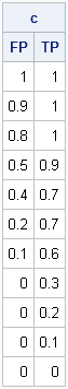
You can call the ROC module with the example data and obtain the points on the ROC curve:
c = ROC(x, y); print c[colname={"FP" "TP"}]; |
Other Equivalent Formulations
As Krzanowski and Hand point out (p. 9), disciplines other than statistics have developed these same ideas independently, but use different names. The health sciences use the term sensitivity to mean the true positive rate. They use specificity to mean the true negative rate. That is why the ROC curve produced by the LOGISTIC procedure has axes that are labeled "1 – specificity" and "sensitivity."
Other disciplines use characteristics of the ROC curve other than the area under the curve (AUC). For example, analysts in finance and economics use the Gini index (p. 27–28), which is simply 2*AUC – 1. Charlie H. calls this the "accuracy ratio" in his blog; see also Murphy Choi's article on the Gini index.

5 Comments
I created a LOGISTIC model with more than 300.000 row.
I would like to creat a ROC curve but PROC LOGISTICS does not give me .
Do you have an idea hoe can I creat this ROC curve ?
Thanks
You can read the documentation for the OUTROC= option in the MODEL statement.
Thanks I will try....
Hi Rick
I need to simulate simulate 4 ROC curves going from 0.15 0.25 0.3 0.35 are above the reference line of a random model.
Could you help me with this ? I need to create these graphs to illustrate a logistic regression model.
Thanks
Jorge Ribeiro
jorgesmithribeiro@yahoo.co.uk
You can post questions like this to the SAS Support Community for Statistical Procedures