In last week's article on how to create a funnel plot in SAS, I wrote the following comment:
I have not adjusted the control limits for multiple comparisons. I am doing nine comparisons of individual means to the overall mean, but the limits are based on the assumption that I'm making a single comparison.
This article discusses how to adjust the control limits (called decision limits in the GLM procedure) to account for multiple comparisons. Because the adjustments are more complicated when the group sizes are not constant, this article treats the simpler case in which each group has the same number of observations. For details on multiple comparisons, see Multiple Comparisons and Multiple Tests Using SAS (the second edition is scheduled for Summer 2011).
Example Data and ANOM Chart
In the funnel plot article, I used data for the temperatures of 52 cars. Each car was one of nine colors, and I was interested in whether the mean temperature of a group (say, black cars) was different from the overall mean temperature of the cars. The number of cars in each color group varied. However, in order to simplify the analysis, today's analysis uses only the temperatures of the first four cars of each color.
You can download the new data and all of the SAS statements used in this article. The following statements create the data and run the SAS/QC ANOM procedure to generate the ANOM chart:
ods graphics on; proc anom data=CarTemp2; xchart Temperature*Color; label Temperature = 'Mean Temperature (F)'; label Color = 'Car Color'; run; |
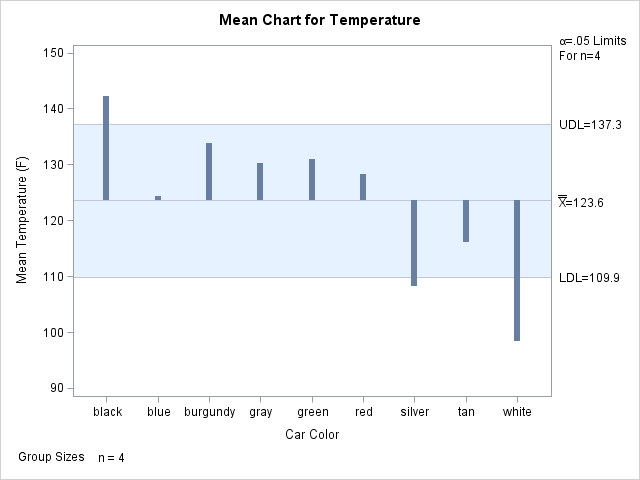
Even for this smaller set of data, it is apparent that black cars are warmer than average and silver and white cars are cooler than average. You can create a similar plot by using the LSMEANS statement in the SAS/STAT GLM procedure.
Computing Decision Limits: An Overview
The formulas for computing decision limits are available in the documentation of the XCHART statement in the ANOM procedure. The decision limits have three components:
- The central value, y, with which you want to compare each individual group mean. Often this is the grand mean of the data.
- A variance term, v, which involves the root mean square error, the number of groups, and the size of each group. This term quantifies the accuracy of the comparisons.
- A multiplier, h, which depends on the significance level, α, and accounts for the multiple comparisons.
Computing the Central Value
The central value is the easiest component to compute. When the group sizes are constant, the central value is merely the overall mean:
proc iml;
use CarTemp2;
read all var {Color Temperature};
close CarTemp2;

/** 1. overall mean **/
y = mean(Temperature); |
This value is 123.6, as shown in the ANOM chart. The ANOM chart compares each individual group mean to this central value.
Computing the Variance Term
The second component in the computation of decision limits is the variance term. This term measures the accuracy you have when comparing group means to the overall mean. (More variance means less accuracy.) The formula involves the mean square error, which in this case is just the average of the sample variances of the nine groups. For convenience, the following statements define a SAS/IML module that computes the average variance:
/** 2. variance term **/
start MSEofGroups(g, x);
   u = unique(g); /** g is group var **/
   nGroups = ncol(u);
   v = j(1, nGroups);
   do i = 1 to nGroups;
      v[i] = var( x[loc(g=u[i])] );
   end;
   return( sum(v)/nGroups );
finish; |
The module is then used to compute the variance term:
MSE = MSEofGroups(Color, Temperature);
nGroups = 9; /** or determine from data **/
size = repeat(4, nGroups); /** {4,4,...,4} **/
v = sqrt(MSE) * sqrt((nGroups-1)/sum(size)); |
Computing the ANOM Multiplier
The final component in forming the ANOM decision limits is the multiplier, h. In elementary statistics, the value 2 (or more precisely, the 0.975 quantile of a t distribution) might be used as a multiplier, but that value isn’t big enough when multiple comparisons are being made. The PROC ANOM documentation states that in a comparison of several group means with the overall mean, the proper value of h is the α quantile of a certain distribution. However, the documentation does not specify how to compute this quantile.
In SAS software you can compute the quantile by using the PROBMC function. I had never heard of the PROBMC function until I started working on this article, but it is similar to the QUANTILE function in that it enables you to obtain quantiles from one of several distributions that are used in multiple comparison computations. (You can also use the PROBMC function to obtain probabilities.)
The following statements compute h for α = 0.05 and for the case of nine groups, each with four observations:
/** 3. multiplier for ANOM **/
alpha = 0.05;
pAnom = 1 - alpha;

/** degrees of freedom for
    pooled estimate of variance **/
df = sum(size)-nGroups;
h = probmc("ANOM", ., pAnom, df, nGroups); |
The main idea is that h is the α quantile of the "ANOM distribution." Although the "ANOM distribution" is not as well-known as the t distribution, the idea is the same. The distribution involves parameters for the degrees of freedom and the number of groups. In the general case (when the group sizes are not constant), the sizes of the groups are also parameters for the distribution (not shown here).
Computing the Decision Limits
All three pieces are computed, so it is easy to put them together to compute the upper and lower decision limits:
/** compute decision limits **/ upperAnom = y + h * v; lowerAnom = y - h * v; print lowerAnom upperAnom; |
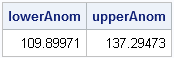
Notice that these values are identical to the values graphed by the ANOM procedure.
Comparing the ANOM Multiplier with Better-Known Multipliers
The computation is finished, but it is interesting to compare the ANOM multiplier with more familiar multipliers from the t distribution.
A classic way to handle multiple comparisons is to use the Bonferroni adjustment. In this method, you divide α by the number of comparisons (9) but continue to use quantiles of the t distribution. By dividing α by the number of groups, you find quantiles that are further in the tail of the t distribution and therefore are larger than the unadjusted values. You can show that the Bonferroni multiplier is a conservative multiplier that will always be larger than the ANOM multiplier.
The following statements compute decision limit multipliers based on an unadjusted t quantile (such as is used for a classical confidence interval for a mean) and on a Bonferroni adjusted quantile. These are printed, along with the multiplier h that was computed previously.
/** compare with unadjusted and Bonferroni multipliers **/
q = quantile("T", 1-alpha/2, df);
qBonf = quantile("T", 1-alpha/2/nGroups, df);
print q qBonf h; |
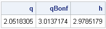
For these data, the Bonferroni multiplier is only about 1% larger than h. You can see that the Bonferroni and ANOM multipliers are about 50% larger than the multiplier based on the unadjusted quantile, which means that the decision limits based on these quantiles will be wider. This is good, because the unadjusted limits are too narrow for multiple comparisons.

1 Comment
Pingback: Visualize the bivariate normal cumulative distribution - The DO Loop