A previous post described a simple algorithm for generating Fibonacci numbers. It was noted that the ratio between adjacent terms in the Fibonacci sequence approaches the "Golden Ratio," 1.61803399.... This post explains why.

In a discussion with my fellow blogger, David Smith, I made the comment "any two numbers (at least one nonzero) can be used to initialize a Fibonacci sequence and the ratio will STILL converge to the golden ratio."

Well, I was only a little bit wrong. Upon further reflection I decided that a better comment would have been "any two POSITIVE numbers." If we consider ALL numbers, including negatives, the correct statement is "any two numbers except those along a particular line through the origin." Which line? It turns out the answer to that question requires reformulating the problem in terms of matrices.

The Origin of Fibonacci Numbers

Fibonacci was a mathematician who was interested in many topics, including population dynamics. A simple model of rabbit reproduction led to the famed Fibonacci sequence. (A nice discussion of this problem is available in a MATLAB e-book by Cleve Moler.) In the Fibonacci sequence, the number of rabbit pairs at time n is determined by sum of the number of pairs at the two preceding units of time:
P_n = P_n-1 + P_n-2.

If you know the initial conditions P₀ and P₁, then the dynamics of the population are completely determined.

In mathematical terms, this is a discrete dynamical system. In matrix terms, the dynamics are determined by iteration of the Fibonacci matrix.

The Fibonacci Matrix

You can use matrices to explore the Fibonacci dynamics for any initial condition. Let F be the 2 x 2 matrix that moves the population forward one unit in time:

proc iml;
F = {1 1, 1 0}; /** F = Fibonacci matrix **/

The complete population dynamics are given by iteration of F. For example, the classical Fibonacci sequence has P₀=1 and P₁=1:

v1 = {1, 1};    /** population at time 0 and 1 **/
v2 = F*v1;      /** population at time 1 and 2 **/
v3 = F*v2;      /** population at time 2 and 3 **/
print v1 v2 v3;

The top number in the table gives the population at each unit of time. A goal of population dynamics is to determine the long-term behavior of the population.

What Happens after Many Iterations?

The matrix F defines a linear system whose dynamics are completely determined by the eigenvalues and eigenvectors of the matrix. You can compute the eigenvalues and eigenvectors for the Fibonacci matrix as follows:

call eigen(val, vect, F);
print val vect;

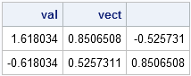
We see that the Fibonacci matrix has one positive eigenvalue. Wait, is that value the GOLDEN RATIO?! Yes, and I'll get back to that fact.

The dynamics induced by iterating this equation are simple:

1. The origin is fixed.
2. The eigenvectors are invariant. Any point on the positive eigenvector iterates to infinity. Any point on the negative eigenvector iterates towards the origin.
3. All other points approach the positive eigendirection as they iterate to infinity.

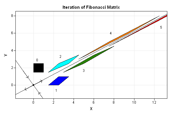
The following image graphically depicts the iteration of a square of initial conditions under iteration of the Fibonacci matrix. The initial conditions are shown in black. Subsequent iterations are shown in blue, cyan, olive green, orange, and red. For reference, the positive and negative eigendirections are also indicated. The SAS/IML Studio program that plots the iterations is available.

The Golden Ratio

Since almost all initial conditions quickly approach the positive eigenvector, the long term dynamics are asymptotically the same as the dynamics on the positive eigenvector. Namely, the value at time n+1 is some multiple of the value at time n. What multiple? Why, the positive eigenvalue, of course! And we have seen that the positive eigenvalue for the Fibonacci matrix is the golden ratio.

Thus, the ratio between numbers in a Fibonacci sequence approaches the golden ratio, and this statement is solely a property of the rule used to define the dynamical system. In particular, the statement is independent of the numbers used to initialize the sequence, as long as the initial conditions are not on the negative eigendirection.

Who knew matrices could be so much fun?