Monte Carlo techniques have many applications, but a primary application is to approximate the probability that some event occurs. The idea is to simulate data from the population and count the proportion of times that the event occurs in the simulated data.

For continuous univariate distributions, the probability of an event is the area under a density curve. The integral of the density from negative infinity to a particular value is the definition of the cumulative distribution function (CDF) for a distribution. Instead of performing numerical integration, you can use Monte Carlo simulation to approximate the probability.

One-dimensional CDFs

In SAS software, you can use the CDF function to compute the CDF of many standard univariate distributions. For example, the statement prob = cdf("Normal", -1) computes the probability that a standard normal random variable takes on a value less than -1.

The CDF function is faster and more accurate than a Monte Carlo approximation, but let's see how the two methods compare. You can estimate the probability P(X < -1) by generating many random values from the N(0,1) distribution and computing the proportion that is less than -1, as shown in the following SAS DATA step

data _NULL_;
call streaminit(123456);
N = 10000;                       /* sample size */
do i = 1 to N;
   x = rand("Normal");           /* X ~ N(0,1) */
   cnt + (x < -1);               /* sum of counts for value less than -1 */
end;
Prob = cdf("Normal", -1);        /* P(x< -1) */
MCEst = cnt / N;                 /* Monte Carlo approximation */
put Prob=;
put MCEst=;
run;

Prob =0.1586552539
MCEst=0.1551

The Monte Carlo estimate is correct to two decimal places. The accuracy of this Monte Carlo computation is proportional to 1/sqrt(N), where N is the size of the Monte Carlo sample. Thus if you want to double the accuracy you need to quadruple the sample size.

Two-dimensional CDFs

SAS provides the PROBBNRM function for computing the CDF of a bivariate normal distribution, but does not provide a built-in function that computes the CDF for other multivariate probability distributions. However, you can use Monte Carlo techniques to approximate multivariate CDFs for any multivariate probability distribution for which you can generate random variates.

I have previously blogged about how to use the PROBBNRM function to compute the bivariate normal CDF. The following SAS/IML statements demonstrate how to use a Monte Carlo computation to approximate the bivariate normal CDF. The example uses a bivariate normal random variable Z ~ MVN(0, Σ), where Σ is the correlation matrix with Σ₁₂ = 0.6.

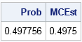
The example computes the probability that a bivariate normal random variable is in the region G = {(x,y) | x<x₀ and y<y₀}. The program first calls the built-in PROBBNRM function to compute the probability. Then the program calls the RANDNORMAL function to generate 100,000 random values from the bivariate normal distribution. A binary vector (group) indicates whether each observation is in G. The MEAN function computes the proportion of observations that are in the region.

proc iml;
x0  = 0.3; y0 = 0.4; rho = 0.6; 
Prob = probbnrm(x0, y0, rho);      /* P(x<x0 and y<y0) */
 
call randseed(123456);
N = 1e5;                           /* sample size */
Sigma = ( 1 || rho)//              /* correlation matrix */
        (rho||  1 );
mean = {0 0};
Z = randnormal(N, mean, Sigma);    /* sample from MVN(0, Sigma) */
group = (Z[,1] < x0 & Z[,2] < y0); /* binary vector */
MCEst = mean(group);               /* = sum(group=1) / N  */
print Prob MCEst;

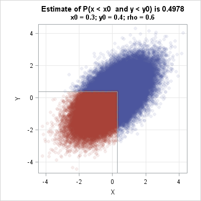
You can use a scatter plot to visualize the Monte Carlo technique. The following statements create a scatter plot and use the DROPLINE statement in PROC SGPLOT to indicate the region G. Of the 100000 random observations, 49750 of them were in the region G. These observations are drawn in red. The observations that are outside the region are drawn in blue.

ods graphics / width=400px height=400px;
title "Estimate of P(x < x0  and y < y0) is 0.4978";
title2 "x0 = 0.3; y0 = 0.4; rho = 0.6";
call scatter(Z[,1], Z[,2]) group=group grid={x y}
     procopt="noautolegend aspect=1"
     option="transparency=0.9  markerattrs=(symbol=CircleFilled)"
     other="dropline x=0.3 y=0.4 / dropto=both;";

Higher dimensions

The Monte Carlo technique works well in low dimensions. As the dimensions get larger, you need to generate a lot of random variates in order to obtain an accurate estimate. For example, the following statements generate 10 million random values from the five-dimensional distribution of uncorrelated normal variates and estimate the probability of all components being less than 0:

d = 5;                         /* dimension */
N = 1e7;                       /* sample size */
mean = j(1, d, 0);             /* {0,0,...,0} */
Z = randnormal(N, mean, I(d)); /* Z ~  MVN (0, I)  */
v0 = {0 0 0 0 0};              /* cutoff values in each component */
ComponentsInRegion = (Z < v0)[,+]; /* number of components in region */
group = (ComponentsInRegion=d);    /* binary indicator vector */
MCEst = mean(group);               /* proportion of obs in region */
print (1/2**d)[label="Prob"] MCEst;

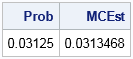
Because the normal components are independent, the joint probability is the product of the probabilities for each component: 1/2⁵ = 0.03125. The Monte Carlo estimate is accurate to three decimal places.

The Monte Carlo technique can also handle non-rectangular regions. For example, you can compute the probability that a random variable is in a spherical region.

The Monte Carlo method is computationally expensive for high-dimensional distributions. In high dimensions (say, d > 10), you might need billions of random variates to obtain a reasonable approximation to the true probability. This is another example of the curse of dimensionality.