There are several ways to simulate multinomial data in SAS. In the SAS/IML matrix language, you can use the RANDMULTINOMIAL function to generate samples from the multinomial distribution. If you don't have a SAS/IML license, I have previously written about how to use the SAS DATA step or PROC SURVEYSELECT to generate multinomial data.

The direct method for simulating multinomial data

The direct method constructs each multinomial observation by simulating the underlying process, which can be thought of as drawing N balls (with replacement) from an urn that contains balls of k different colors. The parameters to the multinomial distribution are N (the number of balls to draw) and (p₁, p₂, ..., p_k), which is a vector of probabilities. Here p_i is the probability of drawing a ball of the ith color and Σ_i p_i = 1.

In the direct method, you simulate one multinomial draw by explicitly generating N balls and counting the number of each color. The distribution of counts (N₁, N₂, ..., N_k) follows a multinomial distribution, where N = Σ_i N_i. The direct method runs quickly if N is small and you simulate a relatively small multinomial sample. For example, when N=100 you can simulate thousands of multinomial observations almost instantly.

The conditional method for simulating multinomial data

If N is large or you plan to generate a large number of observations, there is a more efficient way to simulate multinomial data in the SAS DATA step. It is called the "conditional method" and it uses the fact that you can think of a multinomial draw as being a series of binomial draws (Gentle, 2003, pp. 198-199).

Think about generating the N_i in sequence. The first count, N₁, follows the binomial distribution Bin(p₁, N). If you generate a specific value n₁, then there are N - n₁ items left to draw. The probability of drawing N₂ is p₂ / (1-p₁), which implies that N₂ ~ Bin(p₂ / (1-p₁), N - n₁).

Continue this process. If the first i-1 counts have been drawn, then N_i ~ Bin(N − n₁ - ... - n_i-1, p_i/(1 − p₁ - ... - p_i-1 )). This leads to the following efficient simulation method for multinomial observations:

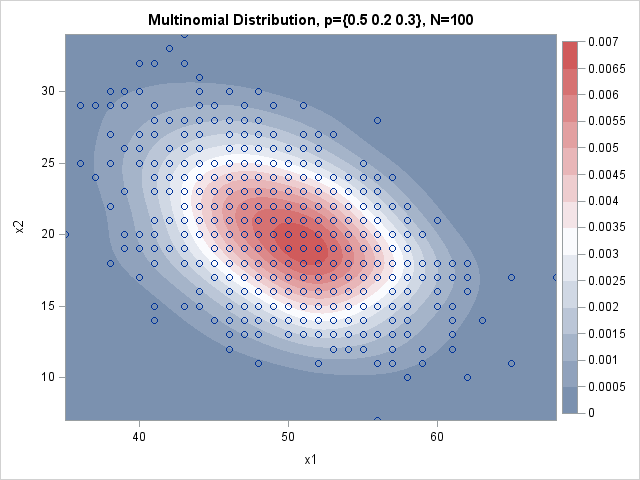
/* generate multinomial sample by using conditional method */
%let SampleSize = 1000;             /* number of observations in MN sample */
%let N = 100;                       /* number of trials in each MN draw */
data MN;
call streaminit(12435);
array probs{3} _temporary_ (0.5 0.2 0.3); /* prob of drawing item 1, 2, 3 */
array x{3};                         /* counts for each item */
do obs = 1 to &SampleSize; 
   ItemsLeft = &N;                  /* how many items remain? */
   cumProb = 0;                     /* cumulative probability */
   do i = 1 to dim(probs)-1;        /* loop over k categories */
      p = probs[i] / (1 - cumProb);
      x[i] = rand("binomial", p, ItemsLeft);     /* binomial draw */
      ItemsLeft = ItemsLeft - x[i]; /* decrement size by selection */
      cumProb = cumProb + probs[i]; /* adjust prob of next binomial draw */
   end;
   x[dim(probs)] = ItemsLeft;       /* remaining items go into last category */
   output;
end;
keep x:;
run;
 
title "Multinomial Distribution, p={0.5 0.2 0.3}, N=100";
proc kde data=MN;
   bivar x1 x2 / bwm=1.5 plots=ContourScatter;
run;

Whereas the direct method requires an inner DO loop that performs N iterations, the conditional method only requires k iterations, where k is the number of categories being drawn. In the example, N=100, whereas k=3. The direct method must generate 100,000 values from the "Table" distribution, whereas the conditional method generates 3,000 values from the binomial distribution.

The graph shows 1,000 observations from the multinomial distribution with N=100 and p={0.5, 0.2, 0.3}. Because of overplotting, you cannot see all 1,000 observations, so the scatterplot is overlaid on a kernel density estimate. The graph shows the counts for the first two categories; the third count is determined by the fact that the counts sum to 100. Notice that the distribution of counts is centered near the expected values x₁=50 and x₂=20.

In summary, if you want to simulate multinomial data by using the SAS DATA step, the algorithm in this article is more efficient than the brute-force direct computation. This algorithm simulates a multinomial vector conditionally as a series of binomial draws.