A heat map is a graphical representation of a matrix that uses colors to represent values in the matrix cells. Heat maps often reveal the structure of a matrix. There are three common applications of visualizing matrices with heat maps:
- Visualizing a correlation or covariance matrix reveals relationships between variables. Chris Hemedinger has written an article that describes how to visualize correlation matrices by using a heat map.
- Visualizing a data matrix reveals outliers, missingness patterns, and more. I will discuss this application in a future blog post.
- The first two applications are usually visualized by using a color ramp with a continuous color gradient. If the matrix contains a small number of discrete values, it is preferable to use a discrete palette of colors. Heat maps with discrete color palettes are useful for visualizing structured covariance matrices and the nonzero pattern of sparse matrices.
This article describes how to use a heat map to visualize matrices that contain a small number of discrete values. (EDIT: As of SAS 9.4m1, there is an easier way to create heat maps of matrices in SAS/IML. See the articles about continuous heat maps and discrete heat maps.)
A structured covariance matrix
In my book Simulating Data with SAS, I simulate data from a repeated-measures model that has a block-diagonal covariance structure. The following SAS/IML statements create a 45 x 45 matrix that consists of nine 5 x 5 blocks:
proc iml; k=5; /* number of repeated measurements */ s=9; /* number of individuals */ B = 1.4*j(k,k,1) + 2*I(k); /* compound symmetric matrix */ R = I(s) @ B; /* block-diagonal matrix */ print R; |
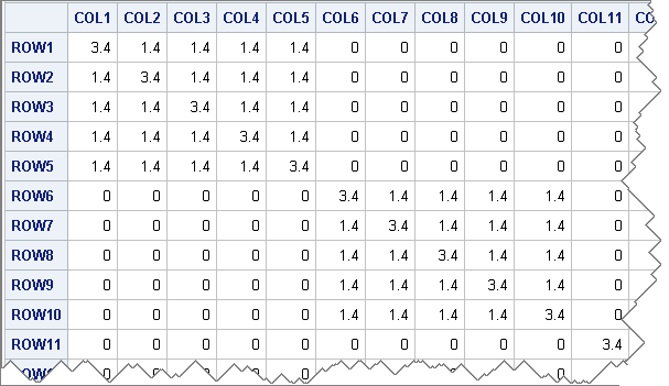
This matrix is too large to easily view in printed form, but you can create a heat map that visualizes the matrix by assigning colors to the three values in the matrix.
Create a data set for the matrix in "long form"
I need to write the SAS/IML matrix to a data set so that it can be read by PROC SGRENDER, which will create the heat map by using a custom GTL template. It turns out that the HEATMAPPARM statement in the GTL language requires that the data set represent the matrix in "long form," which I have discussed in a previous blog post. For specific details, you can download the SAS program that generates the plots in this article.
A template for visualizing a matrix with a small number of unique values
The template to visualize the heat map is straightforward. It contains the following noteworthy features:
- The DYNAMIC statement enables you to specify the names of the data set variables at run time. I like to use this statement so that I can re-use my templates, but you are welcome to hard-code the names of the variables into the template if you prefer.
- The LAYOUT OVERLAY statement specifies three things.
- It specifies the aspect ratio of the plot so that square matrices look square. The aspect ratio interacts with the height and width of the graph as set by the ODS GRAPHICS statement.
- It specifies that the axes are discrete, rather than continuous.
- It specifies the features of the axes to display. For matrices with fewer than 100 rows or columns, I like to display tick marks and values. For larger matrices, I don't.
- The HEATMAPPARM statement creates the heat map from the data.
- The DISCRETELEGEND statement creates a legend that shows the association between the matrix values and the colors.
proc template; define statgraph HeatmapDisc; dynamic _X _Y _Z; begingraph; /* NOTE: Use the TYPE=DISCRETE statements if your version of SAS is before SAS 9.4m3 */ layout overlay/ aspectratio=1 /* optional: for square matrices */ xaxisopts=( /* type=discrete */ discreteopts=(tickvaluefitpolicy=THIN) display=(line ticks tickvalues)) yaxisopts=( /* type=discrete */ discreteopts=(tickvaluefitpolicy=THIN) display=(line ticks tickvalues) reverse=true); heatmapparm x=_X y=_Y colorgroup=_Z / xbinaxis=false ybinaxis=false name="heatmap" primary=true display=ALL; discretelegend "heatmap"; endlayout; endgraph; end; run; proc sgrender data=BlockDiag template=HeatmapDisc; dynamic _X="col" _Y="row" _Z="X"; run; |
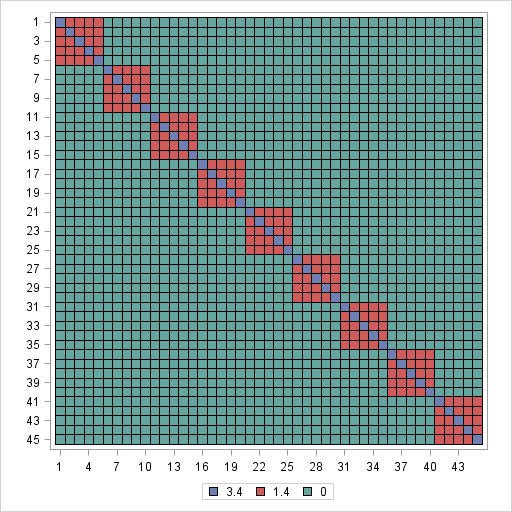
Clearly, the heat map has an advantage over the printed output. The display is smaller, and the global structure of the matrix is readily apparent. At a glance you can see that the matrix is composed of 5 x 5 blocks that contain a large value on the diagonal and smaller values on the off-diagonal. The remaining matrix values are zero.
Visualizing a sparse or binary matrix
Another common application of visualizing matrices is using a heat map to show the structure of a sparse matrix (zero and nonzero cells) or matrices that occur in experimental designs. For example, Hadamard matrices are used to make orthogonal array experimental designs for two-level factors. The following SAS/IML statement creates a 64 x 64 matrix that contains the values 1 and –1:
X = hadamard(64); /* 64 x 64 Hadamard matrix */ |
If you write that matrix (in "long form") to a SAS data set, you can visualize it by using the same GTL template:
proc sgrender data=Hadamard template=HeatmapDisc; dynamic _X="col" _Y="row" _Z="X"; run; |
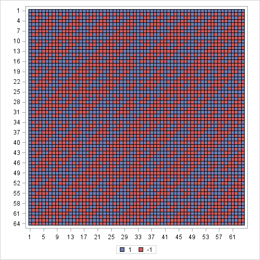
Again, the heat map makes the global structure of the matrix apparent. At a glance you can see that the matrix is composed of two values in a pattern that has many symmetries. Closer inspection reveals that the matrix is symmetric (X = X`) and that each row and column has an equal number of positive and negative values. You can also pick out a "self-similar" structure in the sense that the matrix is composed of four 32 x 32 Hadamard blocks, which are themselves composed of four 16 x 16 Hadamard blocks, and so on, recursively.
In this article, I let the SGRENDER procedure pick default colors for the heat maps. The colors come from the current ODS style, which you can change. Alternatively, you can specify colors in your template, which I will demonstrate in a future blog post.

17 Comments
Aren't the apparent structures only visible because your matrices were built with that structure? If I shuffle the index values (symmetrically), the matrix would still represent the same relationships of the data, but the picture would be very different.
What would I do if I computed pairwise correlations in a large dataset and wanted to discover the structure?
Yes, the structure is apparent because I created it that way. You can use a continuous heat maps to visualize an observed correlation matrix between variables (see Chris's post). There are techniques for permuting the variables so that most of the relationships fall near the diagonal. See Hurley (2004), JCGS.
For correlations between observations (as in this post), you can model a presumed covariance structure by using PROC MIXED. But this assumes that you already know the hierarchical relationships in the data. If you don't, you can try clustering the data and using a heat map to visualize the results. Details and issues are in Wilkinson and Friendly (2009) TAS
How does this scale up to large sparse matrices? I'm talking about matrices with millions of columns and hunderds of thousands of rows, with less than 10 nonzeros per column.
Not very well, considering that the typical computer screen only has 1280-1900 horizontal pixels and only 900-1024 vertical pixels. If you write the graph to HTML ("infinite width and height") you can do better, but I still wouldn't recommend this technique for more than a few thousand rows or columns because global features wouldn't be evident.
Pingback: Hot heat maps
Pingback: Creating a basic heat map in SAS - The DO Loop
Since this tip appeared, I’ve been using heatmaps to help students visualize the covariance structure of a mixed model. The discrete heat map works well, but the default colors are nominal with respect to the covariance value. So I’ve applied a continuous color ramp—which works, but it’s hard to visually distinguish values that are close. To more clearly illustrate the matrix structure, I’d like to use a discrete but sequential color ramp heatmap, so that each value is visible and color reflects an ordinal scale. I’m stumped, though, on whether it can be done without hard-wiring in VALUES in DISCRETEATTRMAP (I am hardly a GTL expert); it would be so nice if it could be more general. Maybe a topic for a future column?
Use the new HEATMAPDISC subroutine:
call heatmapdisc(R);
call heatmapdisc(X);
You can create and use your own sequential color ramp. The new PALETTE function is useful for a small number of categories. For more values, use linear interpolation to create a continuous color ramp, but use it with HEATMAPDISC.
I've recently blogged about the HEATMAPCONT subroutine and plan to blog on HEATMAPDISC in the next few months.
Pingback: A Christmas tree matrix - The DO Loop
Pingback: Creating discrete heat maps in SAS/IML - The DO Loop
Pingback: Visualize missing data in SAS - The DO Loop
Hi,
I have a question concerning heatmaps. Using proc template and proc sgrender, I would like to have a panel of four heatmaps, but doing so, it recomputes the colour response independently for each heatmap, so heatmaps can not be compared. I would like a single scale for all heatmaps. Is there a way to do so ? My codes are :
proc template; /* basic heat map with continuous color ramp */
define statgraph heatmap;
begingraph;
layout lattice/ columns=2 rows=2 rowgutter=10 columngutter=10;
layout overlay
heatmapparm x=order y=trader colorresponse=v1 / /* specify variables at run time */
name="heatmap1" primary=true
xbinaxis=false ybinaxis=false colormodel=(white red darkred)
XENDLABELS=false;
continuouslegend "heatmap1" ;
endlayout;
layout overlay ;
heatmapparm x=order y=trader colorresponse=v2 / /* specify variables at run time */
name="heatmap2" primary=true
xbinaxis=false ybinaxis=false colormodel=(white red darkred)
XENDLABELS=false; /* tick marks based on range of X and Y */
continuouslegend "heatmap2" / location=outside /*valign=bottom*/;
endlayout;
layout overlay /*
xaxisopts=(display=(line ticks tickvalues))
yaxisopts=(display=(line ticks tickvalues))*/;
heatmapparm x=order y=trader colorresponse=V3 / /* specify variables at run time */
name="heatmap3" primary=true
xbinaxis=false ybinaxis=false colormodel=(white red darkred)
XENDLABELS=false; /* tick marks based on range of X and Y */
continuouslegend "heatmap3" / location=outside /*valign=bottom*/;
endlayout;
layout overlay /*
xaxisopts=(display=(line ticks tickvalues))
yaxisopts=(display=(line ticks tickvalues))*/;
heatmapparm x=order y=trader colorresponse=V4 / /* specify variables at run time */
name="heatmap4" primary=true
xbinaxis=false ybinaxis=false colormodel=(white red darkred)
XENDLABELS=false; /* tick marks based on range of X and Y */
continuouslegend "heatmap4" / location=outside /*valign=bottom*/;
endlayout;
endlayout;
endgraph;
end;
run;
proc sgrender data=all template=heatmap;
run;
Thanks
Philippe
Just to add a comment. If I put the same name='heatmap' instead of name='heatmap1', name='heatmap2'.....I have the same scale on all graphs, but the scale is not correct. Seems to be computed only on using the last heatmap.
You can post questions and code at the SAS Support Community. There is a dedicated Graphics Community.
Just answering to my mail :
Just added :
rangeattrmap name="rmap";
range 0 - 1 / rangecolormodel=(white red darkred);
endrangeattrmap;
rangeattrvar attrmap="rmap" var=V1 attrvar=pColor;
rangeattrvar attrmap="rmap" var=V2 attrvar=pColor1;
rangeattrvar attrmap="rmap" var=V3 attrvar=pColor2;
rangeattrvar attrmap="rmap" var=V4 attrvar=pColor3;
ad then calling Pcolor* for each heatmap. It works fine !
For more uses of the RANGEATTRMAP statement, see "Define custom color ramps by using the RANGEATTRMAP statement in GTL"
Thanks Rick, will look at.