Did you know that there is a mathematical formula that simplifies finding the derivative of a determinant? You can compute the derivative of a determinant of an n x n matrix by using the sum of n other determinants. The n determinants are for matrices that are equal to the original matrix except that you modify the i_th row in the i_th matrix by taking its derivative.

This method is especially useful when you want to evaluate the derivative at a point. Without the formula, you need to compute a derivative in symbolic form, compute the derivative (which will require many applications of the product rule!), and then evaluate the derivative of the determinant at the point. By using the formula, you can compute the derivative of individual elements, evaluate n matrices at a point, and then compute the sum of the n numerical determinants.

This article shows the formula and applies it to computing the derivative or structured covariance matrices that arise in statistical models. However, the formula is applicable to any square matrix.

What is the derivative of a determinant?

If A is a square matrix of numbers, the determinant of A is a scalar number. Geometrically, the determinant tells you how the matrix expands or contracts a cube of volume in the domain when it maps the cube into the range. If det(A) > 1, the linear transformation expands volume; if det(A) < 1, the linear transformation contracts volume. Algebraically, the determinant tells you whether the transformation is invertible (det(A) ≠ 0) or is singular (det(A) = 0).

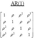
When A is a constant matrix, det(A) is a number. But if some cells in the matrix depend on a parameter, then the determinant is a function of that parameter. A familiar example from statistics is a structured covariance matrix such as the autoregressive AR(1; ρ) correlation matrix. A 4 x 4 correlation matrix with an AR(1) structure is shown to the right. The value of an off-diagonal element is given as a function of the parameter ρ

The AR(1) correlation structure is used in statistics to model correlated errors. If Σ is AR(1) correlation matrix, then its elements are constant along diagonals. The (i,j)th element of an AR(1) correlation matrix has the form Σ[i,j] = ρ^{|i – j|}, where ρ is a constant that determines the geometric rate at which correlations decay between successive time intervals.

The determinant of an AR(1) matrix

Because the AR(1) matrix has a structure, you can compute the determinant in symbolic form as a function of the parameter, ρ. You will get a polynomial in ρ, and it is easy to take the derivative of a polynomial. The computations are long but not complicated. If A is an n x n AR(1) matrix, the following list gives the analytical derivatives of the determinant of A for a few small matrices:

• n=2: d/dρ( det(A) ) = -2 ρ
• n=3: d/dρ( det(A) ) = +4 ρ (ρ² – 1)
• n=4: d/dρ( det(A) ) = -6 ρ (ρ² – 1)²
• n=5: d/dρ( det(A) ) = +8 ρ (ρ² – 1)³

A rowwise method to find the derivative of a determinant

I learned the derivative formula from a YouTube video by Maksym Zubkov ("Derivative of Determinant (for nxn Matrix)"). To find the derivative of the determinant of A, you can compute the determinant of n auxiliary matrices, D_i. The matrix D_i is equal to A except for the i_th row. For the i_th row, you replace the elements of A with their derivatives. Because auxiliary matrices are formed by taking the derivatives of rows, this method is sometimes called the rowwise-method of differentiating the determinant.

For example, let's look at n=2. Typesetting matrices in this blog software is tedious, so I will use the SAS/IML notation where elements on the same row are separated by spaces and commas are used to indicate each row. Thus, the 2 x 2 AR(1) matrix is denoted as
A={1 ρ, ρ 1}.
To compute the derivative of the determinant of A, you form the following auxiliary matrices:

• D₁ = {0 1, ρ 1}. The first row of D₁ contains the derivatives of the first row of A. The determinant of D₁ is det(D₁) = -ρ
• D₂ = {1 ρ, 1 0}. The second row of D₂ contains the derivatives of the second row of A. The determinant is det(D₂) = -ρ
• The derivative of the determinant of A is the sum of the determinants of the auxiliary matrices, which is -2 ρ. This matches the analytical derivative from the previous section.

Flushed with victory, let's try n=3, which is
A = {1 ρ ρ², ρ 1 ρ, ρ² ρ 1}.

• D₁ = {0 1 ρ, ρ 1 ρ, ρ² ρ 1}. The first row of D₁ contains the derivatives of the first row of A. The determinant is det(D₁) = ρ(ρ² – 1).
• D₂ = {1 ρ ρ², 1 0 1, ρ² ρ 1}. The determinant is det(D₂) = 2 ρ(ρ² – 1).
• D₃ = {1 ρ ρ², ρ 1 ρ, 2ρ 1 0}. The determinant of D₃ is ρ(ρ² – 1).
• The derivative of the determinant of A is the sum of the determinants of the auxiliary matrices, which is +4 ρ (ρ² – 1). Again, this matches the analytical derivative from the previous section.

The following figure shows the mathematical formulas for the derivative of the determinant of a 3 x 3 AR(1) matrix:

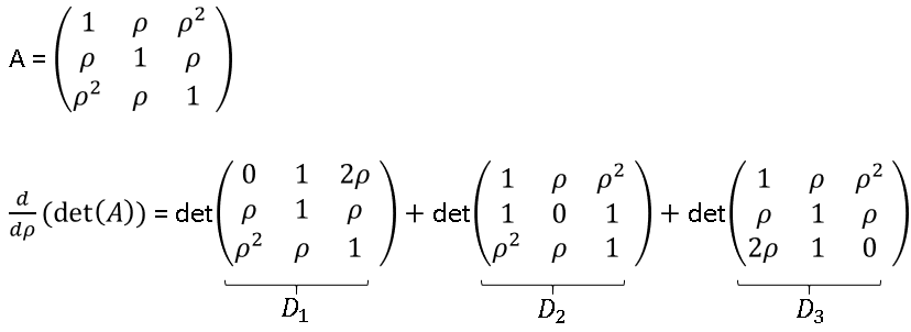
The same method works for any other matrices. To find the derivative of det(A), find the sum of the determinants of the auxiliary matrices, where the i_th auxiliary matrix (D_i) is obtained by taking the derivative of the i_th row of A.

Numerical computation of derivatives of determinants

Let's graph the determinant function for a 3 x 3 AR(1) matrix. You can do this by evaluating the AR(1) matrices for values of ρ in the interval [0, 1] and graphing the determinants as a function of ρ:

proc iml;
/* Construct AR(1; rho):
See https://blogs.sas.com/content/iml/2018/10/03/ar1-cholesky-root-simulation.html 
*/
/* return dim x dim matrix whose (i,j)th element is rho^|i - j| */
start AR1Corr(rho, dim); 
   u = cuprod(j(1,dim-1,rho)); /* cumulative product */
   return( toeplitz(1 || u) );
finish;
 
/* compute the DET at each value of rho and graph the determinant function */
rho = do(0, 1, 0.01);
det = j(1, ncol(rho), .);
do i = 1 to ncol(rho);
   det[i] = det(AR1Corr(rho[i],3));
end;
title "Det(A(rho))";
title2 "A is a 3x3 AR(1) Correlation Matrix";
call series(rho, det) grid={x y} other="refline 0;";

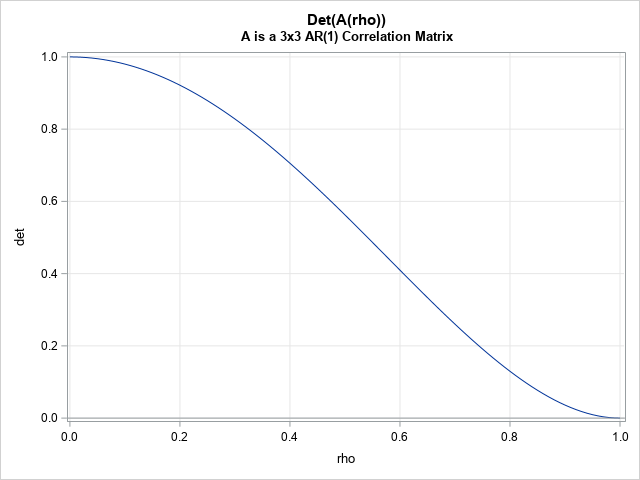
This is the graph of the determinant as a function of the parameter, ρ. From the graph, you can tell that the derivative of this function is 0 at ρ=0 and ρ=1. Furthermore, the derivative is negative on the interval (0, 1) and is most negative near ρ=0.6.

Let's use the derivative formula to compute and graph the derivative of the determinant function:

/* Use the rowwise formula for the derivative of a 3x3 AR(1) matrix:
   The i_th row of D_i is the derivative of the i_th row of A */
start dAR_3D(rho, i);                     /* A=matrix; i = row number */
   A = AR1Corr(rho, 3);
   if      i=1 then A[1,] = {0  1} || 2*rho;   /* derivative of row 1 */
   else if i=2 then A[2,] = {1  0  1};         /* derivative of row 2 */
   else if i=3 then A[3,] = 2*rho || {1  0};   /* derivative of row 3 */
   return( A );
finish;
 
/* compute derivative of DET at each value of rho and graph the derivative function */
rho = do(0, 1, 0.01);
dDet = j(1, ncol(rho), .);
do i = 1 to ncol(rho);
   det = 0;
   do j = 1 to 3;
      det = det + det(dAR_3D(rho[i],j)); /* sum of the determinants of the auxiliary matrices */
   end;
   dDet[i] = det;
end;
 
title "Derivative of Det(A(rho))";
title2 "Sum of Determinants of Auxiliary Matrices";
call series(rho, Ddet) grid={x y} other="refline 0;";

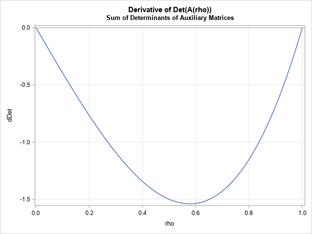
This is the graph of the DERIVATIVE of the determinant as a function of the parameter, ρ. As expected, the derivative is 0 at ρ=0 and ρ=1 and is negative on the interval (0, 1). The derivative reaches a minimum value near ρ=0.6.

Summary

The determinant of a square matrix provides useful information about the linear transformation that the matrix represents. The derivative of the determinant tells you how the determinant changes as a parameter changes. This article shows how to use a rowwise method to compute the derivative of the determinant as the sum of auxiliary matrices. The i_th auxiliary matrix is obtained from the original matrix by differentiating the i_th row. An AR(1) correlation matrix is used as an example to demonstrate the rowwise method.