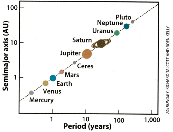
A recent issue of Astronomy magazine mentioned Kepler's third law of planetary motion, which states "the square of a planet's orbital period is proportional to the cube of its average distance from the Sun" (Astronomy, Dec 2016, p. 17). The article included a graph (shown at the right) that shows the period and distance for several planetary bodies. The graph is plotted on a log-log scale and shows that the planetary data falls on a straight line through the origin.

I sometimes see Kepler's third law illustrated by using a graph of the cubed distances versus the squared periods. In a cubed-versus-squared graph, the planets fall on a straight line with unit slope through the origin. Since power transformations and log transformations are different, I was puzzled. How can both graphs be correct?

After a moment's thought, I realized that the magazine had done something very clever. Although it is true that a graph of the squared-periods versus the cubed-distances will CONFIRM the relationship AFTER it has been discovered, the magazine's graph gives insight into how a researcher can actually DISCOVER a power-law relationship in the first place! To discover the values of the exponents in a power-law relationship, log-transform both variables and fit a regression line.

How to discover a power law

Suppose that you suspect that a measured quantity Y is related by a power law to another quantity X. That is, the quantities satisfy the relationship Y^m = A Xⁿ for some integer values of the unknown parameters m and n and constant A. If you have data for X and Y, how can use discover the values of m and n?

One way is to use linear regression on the log-transformed data. Take the logarithms of both size and simplify to obtain log(Y) = C + (n/m) log(X) where C is a constant. You can use ordinary least squares regression to estimate values of the constant C and the ratio n/m.

Planetary periods and distances

For example, let's examine how a modern statistician could quickly discover Kepler's third law by using logarithms and regression. A NASA site for teachers provides the period of revolution (in years) and the mean distance from the Sun (in astronomical units) for several planetary bodies. Some of the data (Uranus, Neptune, and Pluto) were not known to Kepler. The following SAS DATA step reads the data and computes the log (base 10) of the distances and periods:

data Kepler;
input Name $8. Period Distance;
logDistance = log10(Distance);
logPeriod   = log10(Period);
label logDistance="log(Mean Distance from Sun) (AU)"
      logPeriod  ="log(Orbital Period) (Years)";
datalines;
Mercury   0.241   0.387
Venus     0.616   0.723
Earth     1       1
Mars      1.88    1.524
Jupiter  11.9     5.203
Saturn   29.5     9.539
Uranus   84.0    19.191
Neptune  165.0   30.071
Pluto    248.0   39.457
;

The graph in Astronomy magazine plots distances on the vertical axis and periods horizontally, but it is equally valid to flip the axes. It seems more natural to compute a linear regression of the period as a function of the distance, and in fact this how Kepler expressed his third law:

The proportion between the periodic times of any two planets is precisely one and a half times the proportion of the mean distances.

Consequently, the following call to PROC REG in SAS estimates the power relationship between the distance and period:

proc reg data=Kepler plots(only)=(FitPlot ResidualPlot);
   model logPeriod = logDistance;
run;

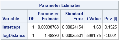
The linear fit is almost perfect. The R² value (not shown) is about 1, and the root mean square error is 0.0005. The table of parameter estimates is shown. The intercept is statistically insignificant. The estimate for the ratio (n/m) is 1.49990, which looks suspiciously like a decimal approximation for 3/2. Thus a simple linear regression reveals the powers used in Kepler's third law: the second power of the orbital period is proportional to the third power of the average orbital distance.

A modern log-log plot of Kepler's third law

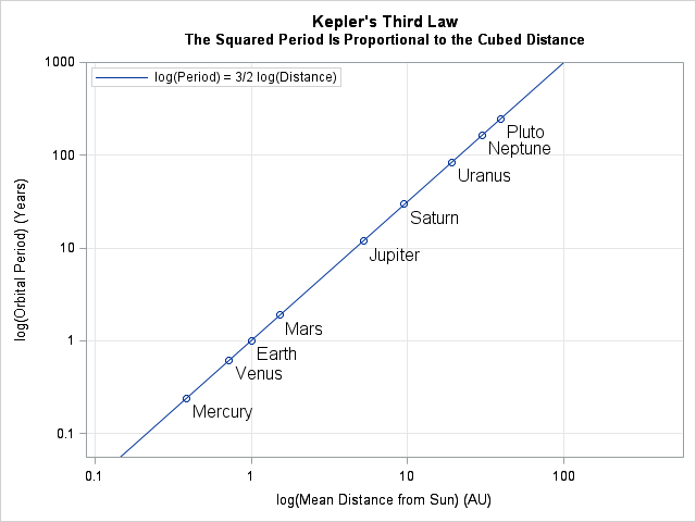
Not only can a modern statistician easily discover the power law, but it is easy to create a scatter plot that convincingly shows the nearly perfect fit. The following call to PROC SGPLOT in SAS creates the graph, which contains the same information as the graph in Astronomy magazine. Notice that I used custom tick labels for the log-scaled axes:

title "Kepler's Third Law";
title2 "The Squared Period Is Proportional to the Cubed Distance";
proc sgplot data=Kepler;
  scatter y=logPeriod x=logDistance / datalabel=Name datalabelpos=bottomright datalabelattrs=(size=12);
  lineparm x=0 y=0 slope=1.5 / legendlabel="log(Period) = 3/2 log(Distance)" name="line";
  yaxis grid values=(-1 0 1 2 3) valuesdisplay=("0.1" "1" "10" "100" "1000") offsetmax=0;
  xaxis grid values=(-1 0 1 2) valuesdisplay=("0.1" "1" "10" "100");
  keylegend "line" / location=inside opaque;
run;

Remark on the history of Kepler's third law

This article shows how a modern statistician can discover Kepler's third law using linear regression on log-transformed data. The regression line fits the planetary data to high accuracy, as shown by the scatter plot on a log-log scale.

It is impressive that Kepler discovered the third law without having access to these modern tools. After publishing his first two laws of planetary motion in 1609, Kepler spent more than a decade trying to find the third law. Kepler said that the third law "appeared in [his]head" in 1618.

Kepler did not have the benefit of drawing a scatter plot on a log-log scale because Descartes did not create the Cartesian coordinate system until 1637. Kepler could not perform linear regression because Galton did not describe it until the 1880s.

However, Kepler did know about logarithms, which John Napier published in 1614. According to Kevin Brown, (Reflections on Relativity, 2016) "Kepler was immediately enthusiastic about logarithms" when he read Napier's work in 1616. Although historians cannot be sure, it is plausible that Kepler used logarithms to discover his third law. For more information about Kepler, Napier, and logarithms, read Brown's historical commentary.