Occasionally on a discussion forum, a statistical programmer will ask a question like the following:
I am trying to fit a parametric distribution to my data. The sample has a long tail, so I have tried the lognormal, Weibull, and gamma distributions, but nothing seems to fit. Please help!!
In general, there is no reason to expect a particular distribution to fit arbitrary data. However, sometimes the person asking the question has a theoretical reason why the model should fit, such as the data are supposed to be "lifetime" data that are part of a reliability or survival analysis.
For several situations that I can remember, the problem occurred because the data distribution was skewed to the left, whereas by convention the usual "named" distributions have positive skewness. The following sample of 50 data values provides an example:
data Sample; input X @@; datalines; 81 91 90 91 87 56 93 80 80 89 93 87 86 58 81 90 82 71 85 94 86 79 82 89 87 87 96 76 77 91 87 67 93 84 90 88 78 92 87 86 61 82 83 92 81 83 87 91 84 72 ; proc univariate data=Sample; histogram X / endpoints=55 to 100 by 5 odstitle="Distribution of Sample Data"; run; |
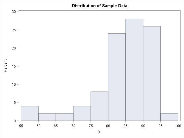
The descriptive statistics from PROC UNIVARIATE (not shown) indicate that the sample skewness is about -1.5. The histogram confirms that the data distribution has negative skewness. Consequently, the lognormal, Weibull, and gamma distributions will not fit these data well.
A transformation that reverses the data distribution
You can transform the data so that the skewness is positive and the long tail is to the right. To do this correctly requires domain-specific knowledge, but the general idea is to apply a linear transformation of the form Y = c – b X for some constants c and b. If you don't want to change the scale of the data, use b = 1.
For example, suppose that the data are the results of an assessment procedure that assigns a value between 0 (bad) and 100 (good) to each item on an assembly line. An alternative way to score each item is to record the number of points that are deducted by the assessment procedure. For the alternative scoring system, low scores are good and high scores are bad. The conversion between the scoring systems is simply Y = 100 – X. The following DATA step creates the new scores and overlays several parametric models that fit the new transformed data:
data Transform; set Sample; Y = 100 - X; run; proc univariate data=Transform; var Y; histogram / endpoints=0 to 45 by 5 odstitle="Distribution of Reversed Data" lognormal(threshold=0) Weibull(threshold=0) gamma(threshold=0); run; |
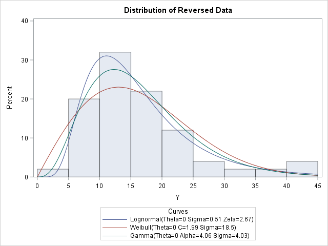
The transformed data has positive skewness. I used knowledge of the data measurements to choose reasonable values for the linear transformation that flips the data distribution. If you know nothing about the data, you could choose c to be any value greater than the maximum data value for X. That guarantees that the transformed data could be modeled by a distribution that has zero for the threshold parameter. Try to choose a transformation for which the new measurements are easy to understand; different values of c will lead to different estimates for the parameters.
In summary, many standard modeling distributions (exponential, lognormal, gamma, Weibull, ...) assume that the data are positively skewed. If your data has negative skewness, try to use a linear transformation to reverse the data before you model it.

4 Comments
Unless there is some rationale for reversing values, I find it rather arbitrary to do so and then hunt for a distribution that fits the data. Instead, I prefer to employ a distribution that can reasonably represent the data as they are collected.
Without knowing more specific information about the data presented here, it appears that values are collected on the range from 0 to 100. The beta distribution is defined on a closed interval and is flexible WRT skewness. That is, the beta distribution can be employed to represent distributions with positive skew, negative skew, or even no skew. If it is correct that values are collected on the range from 0 to 100, then the distribution does indeed have a closed interval. That alone might prompt one to look at the beta distribution. That the data are negatively skewed provides yet another reason to think the beta distribution might be appropriate. I would not that in addition to flexibility in modeling positive or negative skew, the beta distribution is also flexible with regard to kurtosis. Indeed, one can model data with a central modal value and negative kurtosis OR data that have have such positive kurtosis as to be a U-shaped distribution with modes at the extremes.
Estimating the beta distribution to the original (sample) data can be performed employing the code:
proc univariate data=sample;
var x;
histogram / endpoints=55 to 100 by 5
odstitle="Distribution of Sample Data"
beta(theta=0 sigma=100);
run;
Note that theta is the lower bound of the beta distribution and sigma is the LENGTH of the beta distribution (as opposed to the upper bound for the beta distribution). Note, too, that the histogram for X is generated from 55 to 100 by 5 instead of from 0 to 45 by 5. This is consistent with presentation of the histogram for Y from 0 to 45 since Y=100-X. The beta distribution seems to fit reasonably well.
It is interesting to note that since the beta distribution can model any sort of skew and due to its definition on a closed interval, the beta distribution can also be employed for the transformed data. If Y=100-X, and if X follows a beta distribution with theta=0 and sigma=100, then Y also has a beta distribution with theta=0 and sigma=100. Thus, we can examine how well the beta distribution performs at modeling the distribution of X compared to how well the lognormal, Weibull, and gamma do at modeling the transformed data by modeling Y with a beta distribution along with the other three distributions.
proc univariate data=Transform;
var Y;
histogram / endpoints=0 to 45 by 5
odstitle="Distribution of Reversed Data"
lognormal(threshold=0) Weibull(threshold=0) gamma(threshold=0)
beta(theta=0 sigma=100);
run;
Performance of the beta distribution is comparable to performance of the gamma distribution when examined against the transformed data. It seems to provide a reasonable fit to the transformed data. The lognormal distribution would appear to fit the transformed data better. But there is absolutely no a priori reason to think that a lognormal distribution would be appropriate AND the lognormal distribution does not have finite range which is suspected here. Thus, reason for choosing the lognormal distribution is based only on empirical best fit evidence rather than any theoretic arguments. In sample data (particularly if the sample size is small), it should not be surprising to find that the true theoretical distribution is not the best fitting distribution.
I specified parameters theta and sigma of the beta distribution. (Note that theta=0 is the default and didn't really need to be specified above). The beta distribution also has two additional shape parameters, alpha and beta. The relationship between alpha and beta determines both skewness and kurtosis. If beta>alpha, the distribution is skewed right. If alpha>beta, the distribution is skewed left. It may be observed from the estimates provided by the code above that these shape parameters are simply swapped when the transformed data is modeled instead of the sample data. That is, alpha(X)=beta(Y) and beta(X)=alpha(Y) where (X) and (Y) indicate modeling of variables X and Y, respectively.
There is much more that could be written on the beta distribution. But I think the above is sufficient for the problem given here. Hope this is of interest to some.
Hi Dr. Wicklin,
Thank you very much for this post. I have been searching for the most appropriate way to handle my data in preparation for regression analysis, and this seems like a great option. My outcome variables (and their residuals) are negatively skewed beyond what would be appropriate for analysis. I am using multiple imputation, so I don't feel comfortable doing a log-transformation because I am concerned about introducing bias in the imputation. Based on this post, I think my best bet will be to reverse code all of my predictor and outcome variables (so that interpretation will be more intuitive). I will then create generalized linear models and specify a gamma distribution, which will account for the skewness of the now positively coded variables. I am doing my analyses in R rather than SAS but I believe the principles still apply. I considered the advice of the commenter above but I don't think beta analyses will be appropriate for me given my outcome variable is not conceptualized as a proportion or percentage.
I am curious whether you have a publication I can cite that recommends this approach or if you are aware of an article that has implemented this method. I am looking for something to cite in my thesis as an example of why this approach is necessary.
Thank you again,
Kailyn Bare
Wicklin, Rick (2016), “Sometimes You Need to Reverse the Data before You Fit a Distribution,” The DO Loop, 2 Nov. 2016, blogs.sas.com/content/iml/2016/11/02/reverse-data-before-fit-distribution.html.
Thank you for your help!