The skewness of a distribution indicates whether a distribution is symmetric or not. A distribution that is symmetric about its mean has zero skewness. In contrast, if the right tail of a unimodal distribution has more mass than the left tail, then the distribution is said to be "right skewed" or to have positive skewness. Similarly, negatively skewed distributions have long (or heavy) left tails.

Many of us were taught that positive skewness implies that the mean value is to the right of the median. This rule-of-thumb holds for many familiar continuous distributions such as the exponential, lognormal, and chi-square distributions. However, not everyone is aware that this relationship does not hold in general, as discussed in an easy-to-read paper by P. Hipple (2005, J. Stat. Ed.).

In SAS software, the formula for the skewness of a sample is given in the "Simple Statistics" section of the documentation. It is easy to compute the sample skewness Base SAS and in the SAS/IML language. This article shows how.

Use PROC MEANS to compute skewness

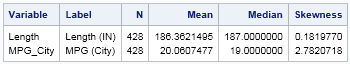
The MEANS procedure supports many univariate descriptive statistics and is my go-to procedure for computing skewness. The following statements compute the mean, median, and skewness for two variables in the Sashelp.Cars data set. The variables are the length of the vehicles and the average fuel economy (miles per gallon) for the vehicles in city driving:

proc means data=sashelp.cars N mean median skew;
var Length MPG_City;
run;

The MEANS procedure does not create graphs, but the following box plots show a distribution of the two variables:

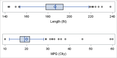
The Length variable has very small skewness (0.18). In the box plot, the diamond symbol represents the mean and the vertical line that divides the box is the median. The box plot indicates that the distribution of the vehicle lengths is approximately symmetric, and that the mean and median are approximately equal.

In contrast, the MPG_City variable has large positive skewness (2.78). The box plot indicates that the data distribution has a short left tail and a long right tail. The mean is to the right of the median, as is often the case for right-skewed distributions.

Computing the skewness in SAS/IML software

The SAS/IML 13.1 release introduced the SKEWNESS function, which makes it easy to compute the skewness for each column of a matrix. The following SAS/IML statements read in the Length and MPG_City variables from the Sashelp.Cars data into a matrix. The SKEWNESS function compute the skewness of each column. The results are identical to the skewness values that were reported by PROC MEANS, and are not shown:

proc iml;
varNames = {"Length" "MPG_City"};
use sashelp.cars;
   read all var varNames into X;
close;
 
skew = skewness(X);
print skew[c=varNames];

I've always thought that it is curious that many "natural" distributions are positively skewed. Many variables that we care about (income, time spent waiting, the size of things,...) are distributions of positive quantities. As such, they are bounded below by zero, but the maximum value is often unbounded. This results in many variables that are positively skewed, but few variables that are negatively skewed. For example, there are 10 numerical variables in the Sashelp.Cars data, and all 10 have positive skewness. Similarly, most of the classical distributions that we learn about in statistics courses are either symmetric or positively skewed.

A canonical example of a negatively skewed distribution is the distribution of grades in a class—especially at schools that have grade inflation. The following data presents hypothetical grades for 30 students who took a test. The test might have been too easy because the median grade is 94.5:

scores = {100 97 67 84 98 100 100 96 87 72 90 100 95 96 89
          100 90 98 85 95 100  96 92 83 90 90 100 66 92 94};
skew = skewness(scores`);
print skew;
 
title "Class Test Scores";
title2 "Skewness = -1.52";
ods graphics / width=400 height=250;
call box(scores) type="HBox";

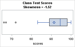
The skewness for this data is -1.52. The box plot indicates that a few students did not score well on the test, although three-quarters of the students received high marks. The box plot shows outliers in the left tail, and the mean is less than the median value.

Why you should care about skewness

Variables that have large skewness (positive or negative) might need special treatment during visualization and modeling. A large skewness value can indicate that the data vary over several orders of magnitude. Some statistics (such as confidence intervals and standard errors) assume that data is approximately normally distributed. These statistics might not be valid for small samples of heavily skewed data.

If you do encounter heavily skewed data, some statisticians recommend applying a normalizing transformation prior to analyzing the data. I have done this in several previous posts, such as the logarithmic transformation of the number of comments made on SAS blogs. In that analysis, the "Number of Responses" variable had a skewness of 4.12 and varied over several orders of magnitude. After applying a log transformation, the new variable had a skewness of 0.5. As a consequence, it was much easier to visualize the transformed data.

I'll end this article by challenging you to examine a mathematical brain teaser. Suppose that you have a data for a positive variable X that exhibits large positive skewness. You can reduce the skewness by applying a log transform to the data. However, there are three common log transformations: You can form Y₂ = log₂(X), Y_e = ln(X), or Y₁₀ = log₁₀(X). Which transformed variable will have the smallest skewness? Mathematically oriented readers can determine the answer by looking at the definition of the sample skewness in the "Simple Statistics" section of the documentation. Readers who prefer programming can use the DATA step to apply the three transformations to some skewed data and use PROC MEANS to determine which transformation leads to the smallest skewness. Good luck!