Prime numbers are strange beasts. They exhibit properties of both randomness and regularity. Recently I watched an excellent nine-minute video on the Numberphile video blog that shows that if you write the natural numbers in a spiral pattern (called the Ulam spiral), then there are certain lines in the pattern that are very likely to contain prime numbers.

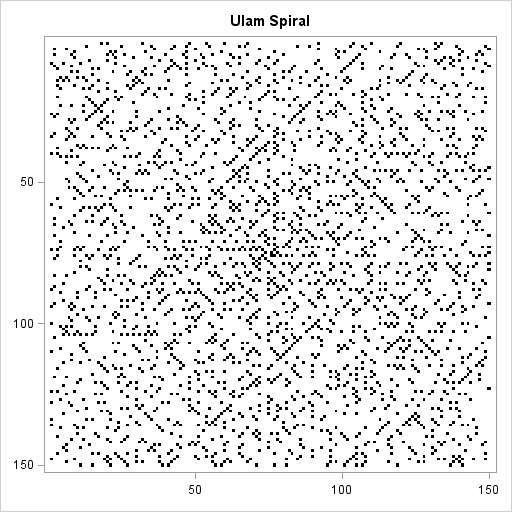
The image to the left shows the first 22,500 natural numbers arranged in the Ulam spiral pattern within a 150 x 150 grid. Cells that contain prime numbers are colored black. Cells that contain composite numbers are colored white. You can see certain diagonal lines with slope ±1 that contain a large number of prime numbers. There are conjectures in number theory that explain why certain lines along the Ulam spiral have a greater density of prime numbers than other lines. (The diagonal lines in the spiral correspond to quadratic equations.)

I don't know enough about prime numbers to blog about the mathematical properties of the Ulam spiral, but as soon as I saw the Ulam spiral explained, I knew that I wanted to generate it in SAS. The Ulam spiral packs the natural numbers into a square matrix in a certain order. This post describes how to construct the Ulam spiral in the SAS/IML matrix language.

The Ulam spiral construction

The Ulam spiral is simple to describe. On a gridded piece of paper, write down the number 1. Then write successive integers as you spiral out in a counter-clockwise fashion, as shown in the accompanying figure.

Although you can stop writing numbers at any time, for the purpose of this post let's assume you want to fill an N x N array with numbers. Notice that when N is even, the last number in the array (N²=4, 16, 36,...), appears in the upper left corner of the array, whereas for odd N, the last number (9, 25, 49,...) appears in the lower right corner. I found this asymmetry hard to deal with, so I created an algorithm that fills the N x N matrix so that the N² term is always in the upper left. For odd values of N, the algorithm rotates the matrix after inserting the elements. I've previously shown that it is easy to write SAS/IML statements that rotate elements in a matrix.

My algorithm constructs the spiral iteratively. Notice that if you have constructed the spiral correctly for an (N–2) x (N–2) array, you can construct the N x N array by adding two vertical columns (first and last) and two horizontal rows (first and last). I call the outer rows and columns a "frame" because they remind me of a picture frame. Given a value for N, you can figure out the starting and ending values of each row and column of the frame. You can use the SAS/IML index creation operator to create each row and column, as shown in the following program:

proc iml;
start SpiralFrame(n);
   if n=1 then return(1);
   if n=2 then return({4 3, 1 2});
   if n=3 then return({9 8 7, 2 1 6, 3 4 5});
   X = j(n,n,.);
   /* top of frame. 's' means 'start'. 'e' means 'end' */
   s = n##2; e = s - n + 2;  X[1,1:n-1] = s:e;
   /* right side of frame */
   s = e - 1; e = s - n + 2; X[1:n-1,n] = (s:e)`;
   /* bottom of frame */
   s = e - 1; e = s - n + 2; X[n,n:2] = s:e;
   /* left side of frame */
   s = e - 1; e = s - n + 2; X[n:2,1] = (s:e)`;
   return( X );
finish;
 
/* test the frame construction */
M2 = SpiralFrame(2);
M4 = SpiralFrame(4);
M6 = SpiralFrame(6);
print M2, M4, M6;

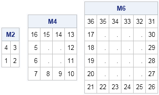
You can see that the M4 matrix fits inside the M6 frame. Similarly, the M2 matrix fits inside the M4 frame.

After writing the code that generates the frames, the rest of the construction is easy. Start by creating the frame of size N. Decrease N by 2 and iteratively create a frame of size N, taking care to insert the (N–2) x (N–2) array into the interior of the existing N x N array. After the array is filled, rotate the array by 180 degrees if N is odd. The following SAS/IML statements implement this algorithm:

start Rot180(m);
   return( m[nrow(m):1,ncol(m):1] );
finish;
 
/* Create N x N integer matrix with elements arranged in an Ulam spiral */
start UlamSpiral(n);
   X = SpiralFrame(n);             /* create outermost frame */
   k = 2;
   do i = n-2 to 2 by -2;          /* iteratively create smaller frames */
      r = k:n-k+1;                 /* rows (and cols) to insert smaller frame */
      X[r, r] = SpiralFrame(i);    /* insert smaller frame */
      k = k+1;
   end;
   if mod(n,2)=1 then return(Rot180(X));
   return(X);
finish;
 
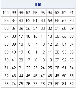
U10 = UlamSpiral(10);              /* test program by creating 10 x 10 matrix */
print U10[f=3.];

You might not have much need to generate Ulam spirals in your work, but this exercise demonstrates several important principles of SAS/IML programming:

• It is often convenient to calculate the first and last element of an array and to use the color index operator (:) to generate the vector.
• Notice that I generated the largest frame first and inserted the smaller frames inside of it. That is more efficient than generating the smaller frames and then using concatenation to grow the matrix.
• In the same way, sometimes an algorithm is simpler or more efficient to implement if your DO loops run in reverse order.

The heat map at the beginning of this article is created by using the new HEATMAPDISC subroutine in SAS/IML 13.1. I will blog about heat maps in a future post. If you have SAS/IML 13.1 and want to play with Ulam spirals yourself, you can download the SAS code used in this blog post.