I'm spoiled by the internet. I've grown so accustomed to being able to instantly find an answer to any query—no matter how obscure—that I am surprised when I don't find what I am looking for.
The other day I was trying to find a mathematical result: a formula for the gradient of the bivariate normal cumulative distribution function (CDF). This does not seem very obscure, but my search came up empty. I searched for "derivatives of bivariate normal probability distribution" and "gradient of multivariate normal cumulative distribution" and a dozen other variations, but nothing revealed a formula. (I found a formula the gradient of the multivariate density function (the PDF), but that wasn't what I needed.)
Eventually I gave up and solved the problem myself. This article shows the formula for the gradient of the bivariate normal cumulative distribution and indicates how to derive it by using calculus.
A formula for the gradient of the bivariate normal CDF
Not everybody is interested in deriving formulas, so I'll jump straight to the result. Assume that the variables have been standardized and have correlation ρ, –1 < ρ < 1. Then the derivatives of the bivariate CDF are as follows:
∂F/∂x = φ(x) Φ(y; ρx, sqrt(1-ρ2))
∂F/∂y = φ(y) Φ(x; ρy, sqrt(1-ρ2))
Here lowercase φ is the univariate standard normal density function and uppercase Φ is the univariate CDF. The expression says that the derivative with respect to x of the bivariate cumulative distribution is equal to a product of two one-dimensional quantities: φ(x), the standard density (PDF) evaluated at x, and Φ(y; ρx, sqrt(1-ρ2)), the CDF at y of a normal distribution with mean ρx and standard deviation sqrt(1-ρ2).
You can compute the gradient in SAS. The following SAS/IML function implements this formula and evaluates the gradient at a few locations in the (x,y) plane:
proc iml;
/* gradient of bivariate normal cumulative distribution */
start GradCDF(x, rho);
   dfdx = pdf("Normal", x[1]) * cdf("Normal", x[2], rho*x[1], sqrt(1-rho##2));
   dfdy = pdf("Normal", x[2]) * cdf("Normal", x[1], rho*x[2], sqrt(1-rho##2));
   return( dfdx // dfdy );
finish;

rho = 0.5;                    /* correlation between X and Y */
pts = { 0 0,
       -1 0,
        0 1};
grad = j(nrow(pts), 2);
do i = 1 to nrow(pts);
   g = GradCDF(pts[i,], rho); /* test the function at a few points */
   grad[i,] = g`;
end;

print (pts||grad)[colname={"x" "y" "dF/dx" "dF/dy"}]; |
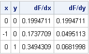
You can confirm that the formulas are correct by using the NLPFDD subroutine to compute finite-difference derivatives of the bivariate normal CDF. For example, the following function evaluates the bivariate CDF by calling the PROBBNRM function in SAS. The numerical finite-difference derivatives that are produced by using the NLPFDD subroutine are identical to the previous output:
start Func(x) global(rho); return( probbnrm(x[1], x[2], rho) ); /* evaluate bivariate CDF at x=(x,y) */ finish; do i = 1 to nrow(pts); call nlpfdd(func, FDDGrad, hessian, "Func", pts[i,]); grad[i,] = FDDGrad; /* numerical approximation of derivatives */ end; print grad; |
Deriving the formula for the gradient of the bivariate normal CDF
This blogging editor isn't great at formatting mathematics, but I'll indicate the main ideas for deriving the gradient of the bivariate normal cumulative distribution function. Recall that the cumulative distribution function is the double integral (with lower limit -∞) of the bivariate normal density:
F(x,y) = C ∫x ∫y f(u,v) du dv
where
f(u, v) = exp( -(u2 - 2ρuv + v2) / (2 sqrt(1-ρ2)) )
and
C = 1/ (2 π sqrt(1-ρ2)) is a normalizing constant.
To compute ∂F/∂x, use the fundamental theorem of calculus to obtain ∂F/∂x = C ∫y f(x,v) dv.
The numerator of the fractional expression inside the exp() function is x2 - 2ρxv + v2. If you complete the square in v, this expression equals (v-ρx)2 + x2(1-ρ)2). The term that does not involve v can come outside the integral sign.
If you rewrite C as (sqrt(2π))–1 * (sqrt(2π) sqrt(1-ρ2))–1 and rearrange the terms, you obtain:
∂F/∂x = φ(x) Φ(y; ρx, sqrt(1-ρ2))
This interesting expression shows once again how the multivariate normal distribution is convenient to work with. The expression says that the derivative with respect to x of the bivariate cumulative distribution is equal to a product of two one-dimensional quantities: the standard univariate density (PDF) at x and a univariate CDF at y. In the univariate CDF, the mean parameter is ρx and the standard deviation parameter is sqrt(1-ρ2).
The formula for the derivative ∂F/∂y is analogous.

11 Comments
Just curious, for what purposes would you need the gradient of the density, as opposed to log-density, where computations simplify considerably? (and are feasible well beyond the normal distribution).
(For the purposes of optimization considering the log-density is equivalent.)
1) As I say in paragraph 2, I'm not computing the gradient of the density, I am computing the gradient of the CUMULATIVE distribution function. The gradient of the density is easy and well known.
2) You are thinking of derivatives with respect to parameters. I am taking derivatives w.r.t x. By the chain rule d/dx( log(F(x,y) ) = 1/f(x,y) * dF/dx. Therefore using the log doesn't prevent needing to know dF/dx.
3) To answer your question, I am finding the gradient because next week I'm going to show how to compute specific contours of the cumulative distribution function.
Thanks a lot for this blog post. My colleagues and I would also like to calculate the gradient of the bivariate standard normal CDF w.r.t. rho, i.e. ∂F/∂ρ. We got: ∂F(x,y,rho)/∂ρ = ∂ ( int_(-infty)^x int_(-infty)^y f( a, b, rho ) db da ) / ∂ρ = int_(-infty)^x int_(-infty)^y ∂ f( a, b, rho ) / ∂ρ ) db da, whereas f( x, y, rho ) is the bivariate standard normal PDF, and we calculated ∂ f( x, y, rho ) / ∂ρ. However, we have not yet managed to solve the double integral so that we can easily compute this integral. Any hints?
Just to clarify, the quantity you are computing is a scalar, not a gradient. Regardless, you can use the QUAD subroutine in SAS/IML software to evaluate double integrals. See the article "Evaluate an iterated integral" and the SAS/IML documentation for the QUAD subroutine, which contains an example that is almost exactly what you need.
Thanks a lot for your immediate response. I prefer to do the integration analytically, because it usually makes the computation much faster and more precise. It seems that the partial derivative of the CDF w.r.t. rho is equal to the PDF:
http://stats.stackexchange.com/questions/77263/bivariate-normal-distribution-and-correlation
Pingback: Symbolic derivatives in SAS - The DO Loop
Shouldn't that formula contain a one-dimensional normal CDF, not a two-dimensional CDF? Remember, after you use the Fundamental Theorem of Calculus, you are left with a one-dimensional integral. I believe that the correct formula should be a product of a one-dimensional PDF and a one-dimensional CDF. The argument to the PDF should be x, and the argument to the CDF should be (v-px)/SQRT(1-p^2). In addition to completing the square, it is necessary to make a change of variables in the CDF integral.
I think you and I have the same formula. In my notation, "Capital Phi" is the one-dimensional CDF with parameters μ and σ. The notation Φ(y; ρx, sqrt(1-ρ^2)) indicates the 1-D normal CDF for variable y, where the parameters μ=ρx and σ=sqrt(1-ρ^2) follow the semicolon. I think from your formula that you were expecting Phi to be the standard CDF. I could have (should have?) used a letter other than Phi to represent the non-standardized cumulative normal distribution, so thanks for pointing out the potential for confusion.
Thank you for straightening me out. Many papers seem to use the "three-argument" format to indicate a 2D CDF. But now that I look, there is no telltale "2" by your CDF, so it must be one-dimensional!
Right. The 2-D standardized CDF might be written as F(x, y; ρ). Mathematicians like to use commas to separate variables and use a semicolon to separate the variables from the parameters. Glad we were able to settle the confusion.
Perhaps you already know about this ... Dr. William Greene (the econometrics guru) has used the derivative of the normal CDF to develop formulae for the marginal effect of variables in a bivariate probit model.