In a previous post, I showed how to solve differential equations in SAS by using the ODE subroutine in the SAS/IML language, which solves initial value problems. This article describes how to draw phase portraits for two classic differential equations: the equations of motion for the simple harmonic oscillator and the pendulum.
A phase portrait for the simple harmonic oscillator
As shown in my previous article, the following statements define the equations of motion for a simple harmonic oscillator and set up some parameters for the ODE subroutine.
proc iml;
/* equations of motion for simple harmonic oscillator, x(0)=x0 and v(0)=v0 */
start SHO(t, z);
  dxdt =  z[2];              /* dx/dt =  v */
  dvdt = -z[1];              /* dv/dt = -x */
  return( dxdt // dvdt );
finish;

h = {1.e-6 1 1e-3}; /* min, max, and initial step size for integration */ |
A phase portrait is a set of parameterized curves in the (x, v) plane that show the dynamics of the differential equation for a variety of initial conditions. The following statements define evenly spaced initial conditions of the form (x0, 0). The trajectories for each initial condition are written to a SAS data set and the SGPLOT procedure is used to visualize the trajectories in the phase plane:
/* Phase portrait: To facilitate using the GROUP= statement in PROC SGPLOT, store
   trajectories in "long" form as a data set with variables IC, T, X, and V. */
x0 = T(do(0.2, 3.0, 0.4)); /* variety of initial positions */
numIC = nrow(x0);
IC = x0 || j(numIC,1,0);   /* each row specifies initial condition (x0, v0) */

/* Choose maximum time length of integration for each IC.
   You might want some trajectories to be longer than others. */
maxT = j(numIC, 1, 6.4);   /* For SHO, all trajectories have period 2*pi  */

names = {"IC" "Time" "x" "v"};
M = {. . . .};  /* establish M as numeric matrix with 4 cols */
create PhasePortrait from M[c=names];  /* open for writing */
do i = 1 to numIC;
   z0 = IC[i,]`;
   t = do(0, maxT[i], 0.2);   /* time intervals for this traj */
   call ode(soln, "SHO", z0, t, h);
   /* fill M with data and write data to SAS data set */
   M = j(ncol(t),1,IC[i,1]) || t` || (z0` // soln`);
   append from M;
end;
close PhasePortrait; |
You can use the SGPLOT procedure to visualize the phase portrait. I don't want to quit PROC IML yet, so I use the SUBMIT and ENDSUBMIT statements to call PROC SGPLOT without leaving IML:
submit; /* the ASPECT= option is a SAS 9.4 feature */ title "Phase Portrait of SHO"; proc sgplot data=PhasePortrait aspect=1 noautolegend; series x=x y=v / group=IC; xaxis grid label="Position"; yaxis grid label="Velocity"; run; endsubmit; |
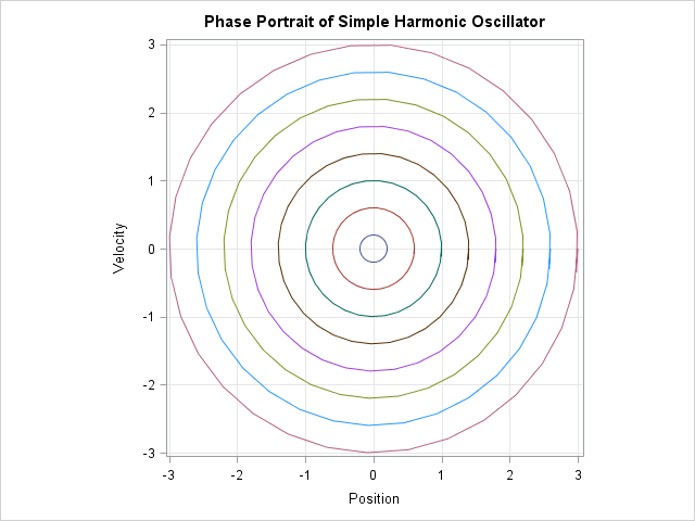
The phase portrait shows that the dynamics of a simple harmonic oscillator are qualitatively similar for all initial conditions. All solutions are sinusoidal. The amplitude of oscillation depends on the initial displacement, but the period of oscillation does not. Each oscillation takes 2π units of time.
A phase portrait for the pendulum
In contrast to the linear oscillator, the equations of motion for the pendulum are nonlinear. Let θ be the angle that the pendulum bob makes with the vertical, so that θ = 0 is the stable equilibrium. Then the domain of the θ variable is [-π, π]. In terms of the angle θ, the equations of motion are defined by the following first-order system:
start Pendulum(t, z); dThetadt = z[2]; /* d(theta)/dt = v (angular velocity) */ dvdt = -sin(z[1]); /* dv/dt = -sin(x) */ return( dThetadt // dvdt ); finish; |
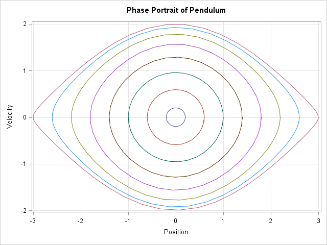
The method for computing the phase portrait of the pendulum is similar to the method for the simple harmonic oscillator. The main difference is that you might want to choose the time of integration to depend on the initial condition. For a pendulum, the period of oscillation depends on the amplitude of oscillation. For small oscillations, the period of the (standardized) pendulum is approximately 2π and the oscillations can be approximated by a simple harmonic oscillator. For large oscillations, however, the period of oscillation is larger. The period is arbitrarily large for initial conditions that are close to the unstable equilibrium at &theta0 = π. Fortunately, the previous code was written to support integration times that vary.
You can download the program that generates phase portraits in SAS. The following graph shows the phase portrait for the pendulum equations. The trajectories near the origin are approximately circles with period of oscillation 2π. As the initial amplitude increases, the shape of the trajectories approach an "eye shape," which is known as a separatrix.
This article has provided two examples of using the ODE subroutine to generate many solutions to a differential equation, each with a different initial condition. When combined with a few tricks in the SAS/IML language, the ODE subroutine enables you to create a phase portrait that shows the qualitative dynamics of the ODE for different initial conditions.
