A histogram displays the number of points that fall into a specified set of bins. This blog post shows how to efficiently compute a SAS/IML vector that contains those counts.

I stress the word "efficiently" because, as is often the case, a SAS/IML programmer has a variety of ways to solve this problem. Whereas a DATA step programmer might sort the data and then loop over all observations to count how many observations are contained in each bin, this algorithm is not the best way to solve the problem in the SAS/IML language.

To visualize the problem, suppose that you are interested in the distribution of the manufacturer's suggested retail price (MSRP) of vehicles in the Sashelp.Cars data set. You can call PROC UNIVARIATE to obtain the following histogram:

proc univariate data=sashelp.cars;
var MSRP;
histogram MSRP / vscale=count barlabel=count
                endpoints=0 to 200000 by 20000;
run;

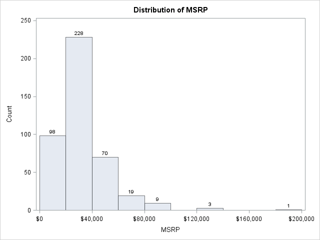
The histogram has a bin width of $20,000 and displays the number of observations that fall into each bin. The bins are the intervals [0, 20000), [20000, 40000), and so on to [180000, 200000).

Constructing Bins

Suppose that you want to use the SAS/IML language to count the number of observations in each bin. The first step is to specify the endpoints of the bins. For these data (prices of vehicles), the minimum value is never less than zero. Therefore, you can use zero as the leftmost endpoint. The endpoint of the rightmost bin is the least multiple of $20,000 that is greater than the maximum vehicle price. Here is one way to define the bins:

proc iml;
use sashelp.cars;               
read all var {MSRP} into v; /** read data into vector v **/
close sashelp.cars;
 
w = 20000;                   /** specify bin width **/
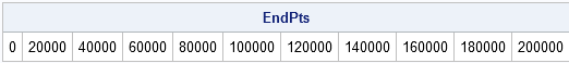
EndPts = do(0, max(v)+w, w); /** end points of bins **/
print EndPts;

Counting Observations in Each Bin

After the bins are defined, you can count the observations that are between the ith and (i + 1)th endpoint. If there are k endpoints, there are k – 1 bins. The following statements loop over each bin and count the number of observations in it:

NumBins = ncol(EndPts)-1;
count = j(1,NumBins,0);      /** allocate vector for results **/
/** loop over bins, not observations **/
do i = 1 to NumBins;      
   count[i] = sum(v >= EndPts[i] & v < EndPts[i+1]); 
end;
 
labels = char(EndPts/1000,3)+"K"; /** use left endpoint of bin as label **/
print count[colname=labels];

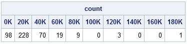
You can compare the SAS/IML counts with the PROC UNIVARIATE histogram to determine that the algorithm correctly counts these data.

The body of the DO loop consists of a single statement. The statement v >= EndPts[i]& v < EndPts[i+1] is a vector of zeros and ones that indicates which observations are in the ith bin. If you call that vector b, you can use b to compute the following quantities:

• You can count the number of observations in the bin by summing the ones: n = sum(b).
• You can compute the percentage of observations in the bin by computing the mean: pct = b[:].
• You can find the indices of observations in the bin by using the LOC function: idx = loc(b). This is useful, for example, if you want to extract those observations in order to compute some statistic for each bin.

Unequally Spaced Bins

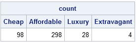
The algorithm uses only endpoint information to count observations. Consequently, it is not limited to equally spaced bins. For example, you might want divide the prices of cars into ordinal categories such as "Cheap," "Affordable," "Luxury," and "Extravagant" by arbitrarily defining price points to separate the categories, as shown in the following statements:

/** count the number of observations in bins of different widths **/
EndPts = {0 20000 60000 100000} || (max(v)+1);
labels = {"Cheap" "Affordable" "Luxury" "Extravagant"};
 
NumBins = ncol(EndPts)-1;
count = j(1,NumBins,0);      /** allocate vector for results **/
do i = 1 to NumBins;      
   count[i] = sum(v >= EndPts[i] & v < EndPts[i+1]); 
end;
 
print count[colname=labels];

In Chapter10 of my book, Statistical Programming with SAS/IML Software, I use this technique to color observations in scatter plots according to the value of a third variable.

I'll leave you with a few questions to consider:

1. Why did I use max(v)+1 instead of max(v) as the rightmost endpoint for the unequally spaced bins?
2. Does this algorithm handle missing values in the data?
3. This algorithm uses half-open intervals of the form [a,b) for the bins. That is, each bin includes its left endpoint, but not its right endpoint. Which parts of the algorithm change if you want bins of the form (a,b]?
4. Notice that the quantity bR = (v < EndPts[i+1]) for i=k is related to the quantity bL = (v >= EndPts[i]) for i=k+1. Specifically, bR equals ^bL. Can you exploit this fact to make the algorithm more efficient?