When you implement a statistical algorithm in a vector-matrix language such as SAS/IML, R, or MATLAB, you should measure the performance of your implementation, which means that you should time how long a program takes to analyze data of varying sizes and characteristics. There are some general tips that can help you eliminate bottlenecks in your program so that your program is fast as lightning! In fact, it is a little bit frightening how quickly you can become an expert in timing.

The following general principles apply regardless of the language that you use to implement the algorithm:

1. Use simulation to construct test data of varying sizes. By simulating data, you can easily vary the size of the size while preserving distributional characteristics. For example, you might want to test an algorithm on data that are normally distributed and contain 25, 50, 75, and 100 thousand observations. (Each language has different techniques to simulate data efficiently. For SAS software, see Simulating Data with SAS.)
2. Vary the distribution of the test data. Concentrate mainly on how the algorithm performs on typical data, but also test examples of "best case" and "worst case" scenarios for which the algorithm might run very quickly or very slowly. If the performance is affected by other factors such as the proportion of outliers or missing values, then include those factors in the study.
3. If possible, construct timing tests that run between 0.1 and 1 seconds. This length is long enough to be reliably measured but short enough that you can run many tests. If you try to time very short intervals (less than a millisecond), you will discover that the operating system constantly performs unrelated background tasks that can interfere with your timings, which leads to noisy measurements. For ultra-short intervals (less than a microsecond), you can encounter an "uncertainty principle" phenomena in which the very act measuring the performance of an algorithm affects the performance that you are trying to measure.
4. To reduce timing noise, call the routine multiple times and report the mean or median. If the performance can vary greatly (±20% or more), report the distribution of times by using quantiles or by displaying a box plot.
5. Use a "burn-in" call to reduce the impact of overhead costs. The first time a routine is called, it might require the operating system to load DLLs or allocate a huge block of memory. When the routine is called a second time, the operating system might have cached the needed information. If so, subsequent calls could be considerably faster than the first.
6. Use a line plot or box plots to present the performance results, where the vertical axis represents time and the horizontal axis represents the size of the data. If the performance characteristics depend on other factors, you can represent those factors by overlaying multiple lines or by constructing a panel of graphs.

Timing the performance of algorithms in SAS/IML

This article is motivated by an R programmer who was trying to find the fastest way (on average) to check whether a vector contains more than one unique value. The programmer was timing the performance of five different methods in R in hopes of finding the fastest. I will use the same example, but will examine only two SAS/IML methods:

• The ALL function in the SAS/IML language tests whether all elements of a vector are equal to some specified value. Thus the expression ALL(x = x[1]) is true only when all elements of a vector are the same.
• The UNIQUE function in the SAS/IML language returns an ordered list of the distinct elements of a vector. Thus the expression (ncol(UNIQUE(x))=1) is true only when a vector contains one distinct value.

The ALL function should be fast to discard non-constant vectors because it a "short-circuiting" operation. That is, as soon as it detects two different values, it returns 0 (false). If you have a vector with 100,000 elements, the ALL function might only examine a small number of elements to determine that the vector is not constant. In contrast, the UNIQUE function should be relatively slow: it always examines all the elements, and it allocates memory to return a sorted list of all unique values.

The following program illustrates many of the best practices. It constructs random binary vectors that contain between 100,000 and 1 million elements. Most elements are 0, but there is a small probability that an element could be 1. Some of the vectors will contain a 1 near the beginning of the vector (the best case for the ALL function), others will contain a 1 near the end (the worst case for ALL).

proc iml;
/* TIP: "Burn-in" by calling each important function once before you start timing */
   x = randfun(N, "Bernoulli", 1/N);   /* Simulate data for size */
   r = all(x = x[1]);          /* method 1: The ALL function */
   r = (ncol(unique(x)) = 1);  /* method 2: The UNIQUE function */
/* end burn-in */
 
sizes = do(2,10,2)*1e5;        /* TIP: choose sizes so test runs in reasonable time */
NReps = 300;                   /* TIP: call functions multiple times */
 
TotalTime = j(ncol(sizes), 2);  /* result matrix: for each size, save average time */
do j = 1 to ncol(sizes);        /* TIP: use vectors of different sizes */
   N = sizes[j];
   x = j(N, 1);
   /* TRICK: estimate time to generate the random vectors; subtract that time later */
   t0 = time();
      do i = 1 to NReps;  call randgen(x, "Bernoulli", 1/N);  end;
   tRand = time() - t0;
 
   /* Method 1: time for NReps calls */
   t0 = time();
   do i = 1 to NReps;
      call randgen(x, "Bernoulli", 1/N);   /* TIP: simulate data for size */
      r = all(x = x[1]);                   /* Method 1: The ALL function */
   end;
   TotalTime[j,1] = time() - t0 - tRand;   /* subtract time to generate random numbers */
 
   /* Method 2: time for NReps calls */
   t0 = time();
   do i = 1 to NReps;
      call randgen(x, "Bernoulli", 1/N);   /* TIP: simulate data for size */
      r = (ncol(unique(x)) = 1);           /* Method 2: The UNIQUE function */
   end;
   TotalTime[j,2] = time() - t0 - tRand;   /* subtract time to generate random numbers */
end;
AvgTime = TotalTime / NReps;               /* compute average time per call */
print AvgTime[c={ALL UNIQUE} r=(putn(sizes,'comma9.')) format=6.4];
 
/* TIP: create a series plot that overlays both curves */
Size = Sizes` // Sizes`;                   /* convert from wide to long data */
Time = AvgTime[,1] // AvgTime[,2];
Group = j(ncol(sizes), 1, "ALL") // j(ncol(sizes), 1, "UNIQUE");
title;
call series(Size, Time) group=Group grid={x y} 
            option="curvelabel" label={"Size", "Average Time per Call"};

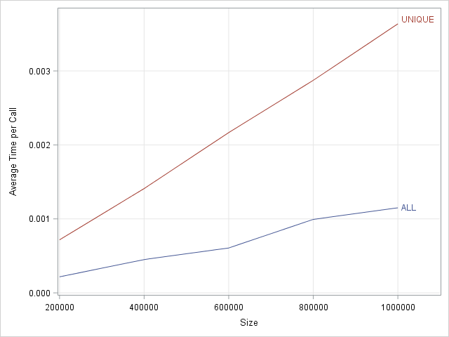
The results are shown to the right. The graph shows the average time to determine whether the elements of a vector of size N are unique for N in the range [1e5, 1e6]. Notice that the graph shows the average time out of 300 different samples of data. As expected, the average time for the ALL function is less than the average time for the UNIQUE function. For the ALL function, some of the tests run almost instantaneously, whereas others require longer run times. The method that calls the UNIQUE function has less variation, although the variation is not shown in this graph.

In terms of absolute time, both methods require only a few milliseconds. In relative terms, however, the ALL method is much faster, and the relative difference increases as the size of the data increases.

Notice that the program demonstrates a useful trick. The ALL function runs much faster than the time required to generate a random vector with a million elements. Therefore the time required to generate a vector and determine whether it is constant is dominated by generating the data. To estimate ONLY the time spent by the ALL and UNIQUE functions, you can either pre-compute the data or you can estimate how long it takes to generate the data and subtract that estimate from the total time. Because this particular test requires generating 300 vectors with 1 million elements, pre-computing and storing the vectors would require a lot of RAM, therefore I used the estimation trick.

In conclusion, when you are timing an algorithm in a vector-matrix language, follow the best practices in this article. The most important tip is to call the method multiple times and plot the average (as I have done here) or plot the distribution of times (not shown). Plotting the average gives you an estimate for the expected time whereas plotting the distribution enables you to estimate upper and lower bounds on the times.

SAS/IML programmers can find additional examples of timing performance in the following articles:

• Compare the performance of algorithms in SAS
• Solving linear systems: Which technique is fastest?
• Remove or keep: Which is faster?