What is kurtosis? What does negative or positive kurtosis mean, and why should you care? How do you compute kurtosis in SAS software?
It is not clear from the definition of kurtosis what (if anything) kurtosis tells us about the shape of a distribution, or why kurtosis is relevant to the practicing data analyst. Mathematically, the kurtosis of a distribution is defined in terms of the standardized fourth central moment. The estimate of kurtosis from a sample also involves a summation that accumulates the fourth powers of a standardized variable. In SAS software, the formula for the sample kurtosis is given in the "Simple Statistics" section of the documentation.
This article presents an intuitive explanation of kurtosis that is often true in practice.
What is kurtosis? Does it make my tail look fat? Share on XWhat is kurtosis?
Let's compute the sample kurtosis for two variables in the Sashelp.Heart data set and see whether the kurtosis values tell us anything about the shape of the data distributions. The variables are AgeAtStart (the age of a patient when he or she entered the study) and Systolic (his or her systolic blood pressure). The following statements call the MEANS procedure to compute estimates for the mean, median, standard deviation, skewness, and kurtosis:
proc means data=sashelp.heart mean median std skew kurtosis; var AgeAtStart Systolic; run; |
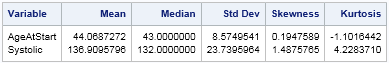
The last column shows that the kurtosis of the AgeAtStart data is negative, whereas the kurtosis of the Systolic data is positive. What does that mean? Well, first recall that whereas the mean, median, and standard deviation are expressed in the same units as the data, kurtosis (like skewness) is a dimensionless quantity. The zero value corresponds to a standard reference situation. For kurtosis, the reference distribution is the normal distribution, which is defined to have a kurtosis of zero. (Technically, I am describing the excess kurtosis, since this is the value returned by statistical software packages. Researchers sometimes consider the full kurtosis, which is 3 more than the excess kurtosis.)
The relationship between kurtosis and the shape of a distribution is complicated, but essentially the kurtosis compares the tails of the distribution to the normal distribution:
- A data distribution with negative kurtosis is often broader, flatter, and has thinner tails than the normal distribution.
- A data distribution with positive kurtosis is often narrower at its peak and has fatter tails than the normal distribution.
Negative kurtosis for a sample indicates that the sample contains many observations that are a moderate distance from the center and few outliers that are far from the center. Kurtosis does not tell us anything about the peak, but in many examples the center of the distribution looks more like a butte or a rounded hilltop than a jutting spire. The canonical distribution that has negative kurtosis is the continuous uniform distribution, which has a kurtosis of –1.2.
In contrast, positive kurtosis indicates one or more outliers that are far from the center. A heavy-tailed distribution has large kurtosis. The canonical distribution that has a large positive kurtosis is the t distribution with a small number of degrees of freedom. Some heavy-tailed distributions have infinite kurtosis.
Graphically testing the kurtosis interpretation
You can run a graphical experiment to see how the shape of the AgeAtStart and Systolic distributions compares with the normal distribution. What would you expect to see if you overlay a normal curve on a histogram of those variables? For the AgeAtStart variable, which has negative kurtosis, you should observe a distribution that has thin tails. For the Systolic variable, you should observe a distribution that has many observations near the mode and has at least one heavy tail. The following statements use PROC SGPLOT to overlay a histogram with a normal curve centered at the median:
ods graphics / width=330px height=250px; proc sgplot data=sashelp.heart noautolegend; histogram AgeAtStart / binwidth=5 binstart=30 showbins; density AgeAtStart / type=normal(mu=43); /* center at median */ run; proc sgplot data=sashelp.heart noautolegend; histogram Systolic / binwidth=10 binstart=80 showbins; density Systolic / type=normal(mu=132); /* center at median */ run; |
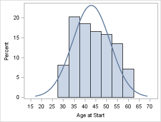
The AgeAtStart variable has negative kurtosis. The histogram for the AgeAtStart variable shows that the distribution is approximately uniform. It does not have a pronounced central peak, and there is substantial mass along most of the range of the data. The distribution appears to be bounded: Apparently the heart study did not accept any patients who were younger than 28 or older than 62. This implies that there are no tails for the population distribution. Overall, the AgeAtStart variable provides a prototypical example of a distribution that has negative kurtosis.
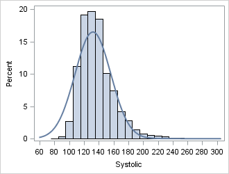
The Systolic variable has positive kurtosis. The histogram of the Systolic variable has a long right tail. There are many patients in the study with systolic blood pressure in the range 120–140. (The American Heart Association calls that range prehypertensive.) Compared to the normal distribution, there are relatively few observations in the ranges (80, 120) and (140, 170). However, the distribution has more extreme observations than would be expected for a normally distributed variable, so the distribution has a fat tail.
Computing kurtosis in SAS software
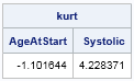
There are three SAS procedures that compute the kurtosis of data distributions. PROC MEANS was used earlier in this article. Use PROC UNIVARIATE when you want to fit a univariate model to the data. PROC IML includes the KURTOSIS function in SAS/IML 13.1, as shown in the following example:
proc iml;
varNames = {"AgeAtStart" "Systolic"};
use Sashelp.Heart;  read all var varNames into X;  close Sashelp.Heart;

kurt = kurtosis(X);
print kurt[colname=varNames]; |
Intuitive interpretation of kurtosis
The relationship between kurtosis and the shape of the distribution are not mathematical rules, they are merely intuitive ideas that often hold true for unimodal distributions. If your distribution is multimodal or is a mixture of distributions, these intuitive rules might not apply.
There have been many articles about kurtosis and its interpretation. Balanda and MacGillivray (1988, TAS) give examples of three different densities that each have the same kurtosis value but that look very different. They conclude that "because of the averaging process involved in its definition, a given value of [kurtosis]can correspond to several different distributional shapes" (p. 114).
They recommend that kurtosis be defined as "the location- and scale-free movement of probability mass from the shoulders of a distribution into its center and tails. In particular, this definition implies that peakedness and tail weight are best viewed as components [emphasis mine]of kurtosis.... This definition is necessarily vague because the movement can be formalized in many ways" (p. 116). In other words, the peaks and tails of a distribution contribute to the value of the kurtosis, but so do other features.
In contrast, Westfall (2014) is adamant that "kurtosis tells you virtually nothing about the shape of the peak—its only unambiguous interpretation is in terms of tail extremity." Westfall presents three distributions that have vastly different peak shapes, but the same kurtosis.
Because the kurtosis is a non-robust statistic, a single outlier can greatly affect the kurtosis. For example, if you choose 999 observations from a normal distribution, the sample kurtosis will be close to 0. However, if you add a single observation that has the value 100, the sample kurtosis jumps to more than 800!
What is kurtosis? Kurtosis is not an easy statistic to interpret, especially for multimodal distributions. However, the intuitive notions in this article hold true for many unimodal data distributions that arise in practice. In essence, kurtosis tells you about the fatness of the tails of a probability distribution, relative to the normal distribution. Positive kurtosis means more outliers than normality; negative kurtosis means fewer outliers.

9 Comments
THE PAPER BY BALANDA ET AL IS NOT FREELY AVAILABLE...
Here is an alternative paper that uses PROC IML...
http://www.lexjansen.com/nesug/nesug98/stat/p105.pdf
Thanks! For some reason Kurtosis has been on my mind recalling long ago stats classes. This is a very helpful, simple --and therefore probably took some time to write-- explanation. It's headed to my onenote file.
Bil
Random Question
Are you aware of any Goal Seeking Solutions ( similar to Solver in Excel ) that can be implemented in PROC IML?
Thank you in anticipation.
Regards
You can solve for the optimal value of a function by using the Nonlinear Programming (NLP) functions in SAS/IML. I've written several blog posts about optimization.
Hello,
very good explanation of the meaning of kurtosis. Thanks a lot.
Annette
The "peakedness" definition of kurtosis is by now officially of historical note only and not useful as a descriptor.
Also, the fact that kurtosis is sensitive to outliers *is* the point of kurtosis. It measures outliers only, and nothing about the peak.
Westfall, P.H. (2014). Kurtosis as Peakedness, 1905 – 2014. R.I.P. The American Statistician, 68, 191–195.
Pingback: The relationship between skewness and kurtosis - The DO Loop
Pingback: Goodness-of-fit tests: A cautionary tale for large and small samples - The DO Loop
Pingback: The sample skewness is a biased statistic - The DO Loop