In the classic textbook by Johnson and Wichern (Applied Multivariate Statistical Analysis, Third Edition, 1992, p. 164), it says:

All measures of goodness-of-fit suffer the same serious drawback. When the sample size is small, only the most aberrant behaviors will be identified as lack of fit. On the other hand, very large samples invariably produce statistically significant lack of fit. Yet the departure from the specified distributions may be very small and technically unimportant to the inferential conclusions.

In short, goodness-of-fit (GOF) tests are not very informative when the sample size is very small or very large.

I thought it would be useful to create simulated data that demonstrate the statements by Johnson and Wichern. Obviously I can't show "all measures of goodness-of-fit," so this article uses tests for normality. You can construct similar examples for other GOF tests.

Small data: Only "aberrant behaviors" are rejected

As I showed last week, the distribution of a small sample can look quite different from the population distribution. A GOF test must avoid falsely rejecting the bulk of these samples, so the test necessarily rejects "only the most aberrant behaviors."

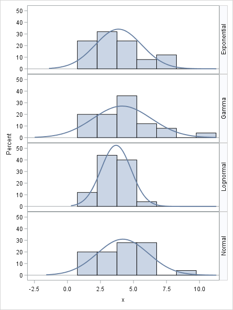
To demonstrate how GOF tests work with small samples, let's generate four samples of size N=25 from the following populations:

• A normal N(4,2) distribution. The population mean and standard deviation are 4 and 2, respectively.
• A gamma(4) distribution. The population mean and standard deviation are 4 and 2, respectively.
• A shifted exponential(2) distribution. The population mean and standard deviation are 4 and 2, respectively.
• A lognormal(1.25, 0.5) distribution. The population mean and standard deviation are 3.96 and 2.11, respectively.

The following SAS DATA step creates the four samples. The Distribution variable identifies the observations in each sample. You can use the SGPANEL procedure to visualize the sample distributions and overlay a normal density estimate, as follows:

data Rand;
call streaminit(1234);
N = 25;
do i = 1 to N;
   Distribution = "Normal     ";
   x = rand("Normal", 4, 2);   output;
   Distribution = "Gamma      ";
   x = rand("Gamma", 4);       output;
   Distribution = "Exponential";
   x = 2 + rand("Expo", 2);    output;
   Distribution = "Lognormal  ";
   x = rand("Lognormal", 1.25, 0.5); output;
end;
run;
 
proc sgpanel data=Rand;
  panelby Distribution / rows=4 layout=rowlattice onepanel novarname;
  histogram x;
  density x / type=normal;
run;

We know that three of the four distributions are not normal, but what will the goodness-of-fit tests say? The NORMAL option in PROC UNIVARIATE computes four tests for normality for each sample. The following statements run the tests:

ods select TestsForNormality;
proc univariate data=Rand normal;
  class Distribution;
   var x;
run;

The results (not shown) are that the exponential sample is rejected by the tests for normality (at the α=0.05 level), but the other samples are not. The samples are too small for the test to rule out the possibility that the gamma and lognormal samples might actually be normal. This actually makes sense: the distribution of these samples do not appear to be very different from some of the normal samples in my previous blog post.

Large samples and small deviations from fit

As Johnson and Wichern said, a large sample might appear to be normal, but it might contain small deviations that cause a goodness-of-fit test to reject the hypothesis of normality. Maybe the tails are a little too fat. Perhaps there are too many or too few outliers. Maybe the values are rounded. For large samples, a GOF test has the power to detect these small deviations and therefore reject the hypothesis of normality.

I will demonstrate how rounded values can make a GOF test reject an otherwise normal sample. The following DATA step creates a random sample of size N=5000. The X variable is normally distributed; the R variable is identical to X except values are rounded to the nearest tenth.

data RandBig;
call streaminit(1234);
N = 5000;
do i = 1 to N;
   x = rand("Normal", 4, 2);
   r = round(x, 0.1);        /* same, but round to nearest 0.1 */
   output;
end;
run;

There is little difference between the X and R variables. The means and standard deviations are almost the same. The skewness and kurtosis are almost the same. Histograms of the variables look identical. Yet because the sample size is 5000, the GOF tests reject the hypothesis of normality for the R variable at the 95% confidence level. The following call to PROC UNIVARIATE computes the analysis for both X and R:

ods select Moments Histogram TestsForNormality;
proc univariate data=RandBig normal;
var x r;
histogram x r / Normal;
run;

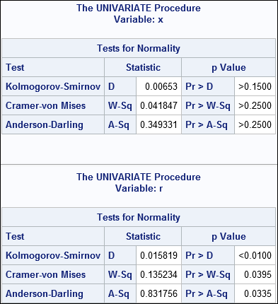
Partial results are shown. The first table is for the variable X. The goodness-of-fit tests fail to reject the null hypothesis, so we correctly accept that the X variable is normally distributed. The second table is for the variable R. The GOF tests reject the hypothesis that R is normally distributed, merely because the values in R are rounded to the nearest 0.1 unit.

Rounded values occur frequently in practice, so you could argue that the variables R and X are not substantially different, yet normality is rejected for one variable but not for the other.

And it is not just rounding that can cause GOF tests to fail. Other small and seemingly innocuous deviations from normality would be similarly detected.

In conclusion, be aware of the cautionary words of Johnson and Wichern. For small samples, goodness-of-fit tests do not reject a sample unless it exhibits "aberrant behaviors." For very large samples, the GOF tests "invariably produce statistically significant lack of fit," regardless of whether the deviations from the target distributions are practically important.