My last blog post described three ways to add a smoothing spline to a scatter plot in SAS. I ended the post with a cautionary note:
From a statistical point of view, the smoothing spline is less than ideal because the smoothing parameter must be chosen manually by the user.
This means that you can specify a smoothing spline parameter that appears to fit the data, but the selection is not based on an objective criterion. In contrast, SAS software supports several other methods for which the software can automatically choose a smoothing parameter that maximizes the goodness of fit while avoiding overfitting. This article describes penalized B-splines loess curves, and thin-plate splines.
Penalized B-splines
You can fit penalized B-splines to data by using the TRANSREG procedure or by using the PBSPLINE statement in the SGPLOT procedure. The TRANSREG procedure enables you to specify many options that control the fit, including the criterion used to select the optimal smoothing parameter. The TRANSREG procedure supports the corrected Akaike criterion (AICC), the generalized cross-validation criterion (GCV), and Schwarz’s Bayesian criterion (SBC), among others. These criteria try to produce a curve that fits the data well, but does not interpolate or overfit the data. The default criterion is the AICC.
To illustrate fitting a smooth curve to a scatter plot, I'll use the SasHelp.enso data set, which contains data on the "southern oscillation," a cyclical phenomenon in atmospheric pressure that is linked to the El Niño and La Niña temperature oscillations in the Pacific Ocean. (ENSO is an acronym for El Niño-Southern Oscillation.) The ENSO data is analyzed in an example in the PROC TRANSREG documentation.
The following statements fit a penalized B-spline to the ENSO data:
proc transreg data=sashelp.enso; model identity(pressure) = pbspline(year); /* AICC criterion */ run; |
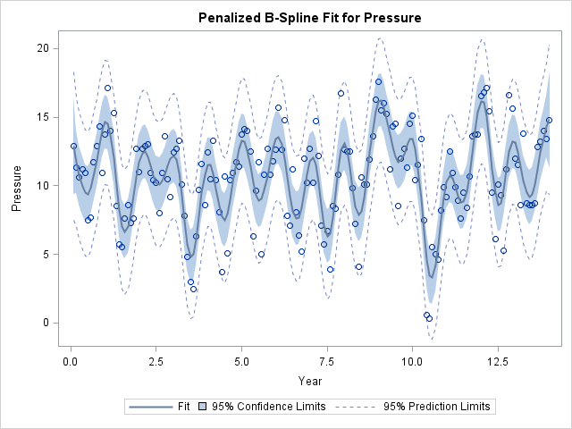
The data shows an oscillation of pressure in a yearly cycle. There are 14 peaks and valleys in this 14-year time series, which correspond to 14 winters and 14 summers.
Loess curves
A loess curve is not a spline. A loess model at x uses a local neighborhood of x to compute a weighted least squares estimate. The smoothing parameter is the proportion of data in the local neighborhood: a value near 0 results in a curve that nearly interpolates the data whereas a value near 1 is nearly a straight line. You can fit loess curves to data by using the LOESS procedure or by using the LOESS statement in the SGPLOT procedure. The LOESS procedure enables you to specify many options that control the fit, including the criterion used to select the optimal smoothing parameter. The LOESS procedure supports the AICC and GCV criteria, among others. The default criterion is the AICC.
The default loess fit to the ENSO data is computed as follows:
ods select FitSummary CriterionPlot FitPlot; proc loess data=sashelp.enso; model pressure = year; run; |

The loess curve looks different than the penalized B-spline curve. The loess curve seems to contain irregularly spaced peaks that are 4–7 years apart. This is the El Niño oscillation cycle, which is an irregular cycle. The selected smoothing parameter is about 0.2, which means that about one-fifth of the observations are used for each local neighborhood during the estimation.
Earlier I said that the LOESS and TRANSREG procedures automatically choose parameter values that optimize some criterion. So why the difference in these plots? The answer is that the criterion curves sometimes have local minima, and for the ENSO data the LOESS procedure found a local minimum that corresponds to the El Niño cycle. The curve that shows the AICC criterion as a function of the smoothing parameter is shown below:
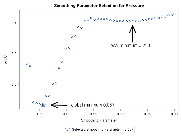
The LOESS procedure supports several options that enable you to explore different ranges for the smoothing parameter or to search for a global minimum. I recommend using the PRESEARCH option in order to increase the likelihood of finding a global minimum. For example, for the ENSO data, the following call to PROC LOESS finds the global minimum at 0.057 and produces a scatter plot smoother that looks very similar to the penalized B-spline smoother.
proc loess data=sashelp.enso; model pressure = year / select=AICC(presearch); run; |
Smoothers with the SGPLOT procedure
Because the loess and penalized B-spline smoothers work well for most data, the SGPLOT procedure supports the PBSPLINE and LOESS statements for adding smoothers to a scatter plot. By default the statements also add the scatter plot markers, so use the NOMARKERS options if you are overlaying a smoother on an existing scatter plot:
proc sgplot data=sashelp.enso; pbspline x=year y=pressure; /* also draws scatter plot */ loess x=year y=pressure / nomarkers; /* uses PRESEARCH option */ run; |
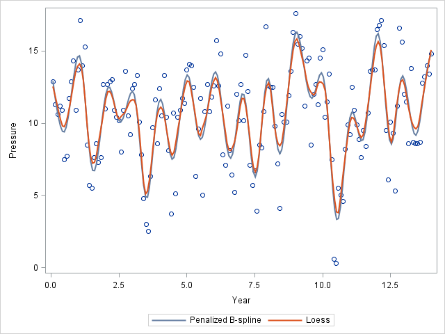
As you can see, the two smoothers produce very similar results on the ENSO data. That is often the case, but not always.
Thin-plate splines
I'm not going to shows examples of every nonparametric regression procedure in SAS, but I do want to mention one more. A thin-plate spline yet another spline that can be used to smooth data. The TPSPLINE procedure supports the GCV criterion for the automatic selection of the smoothing parameter. For the ENSO data, the TPSPLINE procedure produces a smoother the reveals the annual pressure cycle and is very similar to the previous curves:
ods select FitStatistics CriterionPlot FitPlot; proc tpspline data=sashelp.enso; model pressure = (year); run; |
In conclusion, SAS software provides several ways to fit a smoother to data. The procedures mentioned in this article can automatically select a smoothing parameter that satisfies some objective criterion which balances goodness of fit with model parsimony. Do you have a favorite smoother? Let me know in the comments.

14 Comments
Another good post.
Some of this is in my upcoming talk at SGF.
Dear Rick,
thank you very much for pointing this out. Some months ago I was in need for a smoothing tool with an automated selection of the smoothing parameter and chose PROC GLIMMIX. This prcedure has a smoothing option in the RANDOM Statement which uses the similarity between mixed models and penalized splines. I liked this option because it gives you also a statistical test for the need of smoothing (via the COVTEST statement) and you get pointwise confidence intervals for the smooth line.
Here's the code for the ENSO data:
proc glimmix data=sashelp.enso;
model pressure = ;
random year / type=rsmooth;
covtest 'Smoothing' indep;
output out=out_enso pred=p lcl=lcl ucl=ucl;
run;
proc sgplot data=out_enso;
scatter x=year y=pressure;
series x=year y=lcl;
series x=year y=p;
series x=year y=ucl;
run;
Thanks for the code and suggestion. Yes, radial basis functions are useful for smoothing of random effects and revealing trends. For these data the radial smoothers oversmooth the data and do not find the underlying ENSO cycles.
In PROC SGPLOT, I like to use the BAND statement for confidence limits:
band x=year upper=ucl lower=lcl;
Dear Rick,
you're right, you would probably not use the PROC GLIMMIX smoother for the ENSO example because you expect periodic cycles in these data. We were interested in trend changes in standardized incidence ratios for secondary cancers (see citation below) and PROC GLIMMIX worked fine here.
Rusner C et al. Risk of second primary cancers after testicular cancer in East and West Germany: A focus on contralateral testicular cancers. Asian J Androl. 2013 Dec 23. doi: 10.4103/1008-682X.122069. [Epub ahead of print]
A colleague pointed out that you can use the PARMS statement to control the initial guess for the parameter values. This will enable the radial smoother to pick up various cycles, as follows:
Pingback: What is loess regression? - The DO Loop
Pingback: Ahh, that's smooth! Anti-aliasing in SAS statistical graphics - The DO Loop
Pingback: Three ways to add a smoothing spline to a scatter plot in SAS - The DO Loop
Pingback: On the SMOOTHCONNECT option in the SERIES statement - The DO Loop
Pingback: Beware of repeated values in loess models - The DO Loop
Thanks a lot for this great illustration! Can you suggest a method that allows group comparisons? To be more specific: We have a dataset obtained from a Randomized Control Trial, and there are 4 to 6 groups to compare. In each group, we want to use the LOESS procedures you illustrated here.
Do you mean visually compare the smoothers? If so, you can use the GROUP= option on the LOESS statement to display a curve for each group:
Thanks a lot for the code! Visual comparison would be helpful, but I'm looking for a method that can statistically test the model parameters of smoothers across multiple groups. For example, let's consider a 2-way ANOVA design, I want to fit LOESS models for each group and do a statistical test the differences across the groups (instead of comparing group means in a normal ANOVA). Do you have any suggestion for my situation?
I do not know how to do "a statistical test for the differences" between two arbitrary curves. For linear curves, you can ask whether the slopes and intercepts are different. For a general nonlinear parametric curve, you might be able to test whether the parameters are the significantly different. But I don't think your question makes sense for a LOESS curve, which is nonparametric. You could estimate the Root-MSE between two curves, but I don't know how to use the result in a statistical test for the difference. Statistical tests for a null hypothesis are based on knowing the distribution of the sampling distribution of the test statistic under the null.