"I think that my data are exponentially distributed, but how can I check?"

I get asked that question a lot. Well, not specifically that question. Sometimes the question is about the normal, lognormal, or gamma distribution. A related question is "Which distribution does my data have," which was recently discussed by John D. Cook on his blog.

Regardless of the exact phrasing, the questioner wants to know "What methods are available for checking whether a given distribution fits the data?" In SAS, I recommend the UNIVARIATE procedure. It supports three techniques that are useful for comparing the distribution of data to some common distributions: goodness-of-fit tests, overlaying a curve on a histogram of the data, and the quantile-quantile (Q-Q) plot. (Some people drop the hyphen and write "the QQ plot.")

• Goodness-of-fit tests are available by using the HISTOGRAM statement in the UNIVARIATE procedure. There are entire books written about goodness-of-fit tests. A good introduction is given by Stephen's (1974) JASA article.
• The HISTOGRAM statement also overlays the best-fitting density curve on a histogram of the data. Often this involves maximum likelihood estimation. Overlaying a curve on a histogram can be informative, but the apparent fit is affected by the way that the data are binned. Small changes in the choice of the histogram bins can make a big difference in whether the overlaid curve seems to fit the data.
• My favorite technique for comparing the distribution of data with a "named" distribution is the Q-Q plot. You can use the QQPLOT statement in PROC UNIVARIATE to create a Q-Q plot for about a dozen built-in distributions, but it is also straightforward to create the data for a Q-Q plot for any distribution for which you can compute the quantile (inverse CDF) function. You can interpret the Q-Q plot to investigate how the empirical distribution of your data follows or deviates from a theoretical distribution. If the points of a Q-Q plot lie on or near a line, then that is evidence that the data distribution is similar to the theoretical distribution.

Constructing a Q-Q Plot for any distribution

The UNIVARIATE procedure supports many common distributions, such as the normal, exponential, and gamma distributions. In SAS 9.3, the UNIVARIATE procedure supports five new distributions. They are the Gumbel distribution, the inverse Gaussian (Wald) distribution, the generalized Pareto distribution, the power function distribution, and the Rayleigh distribution.

But what if you want to check whether your data fits some distribution that is not supported by PROC UNIVARIATE? No worries, creating a Q-Q plot is easy, provided you can compute the quantile function of the theoretical distribution. The steps are as follows:

1. Sort the data.
2. Compute n evenly spaced points in the interval (0,1), where n is the number of data points in your sample.
3. Compute the quantiles (inverse CDF) of the evenly spaced points.
4. Create a scatter plot of the sorted data versus the quantiles computed in Step 3.

If the data are in a SAS/IML vector, the following statements carry out these steps:

proc iml;
y = {1.7, 1.0, 0.5, 3.5, 1.9, 0.7, 0.4, 
     5.1, 0.2, 5.6, 4.6, 2.8, 3.8, 1.4, 
     1.6, 0.9, 0.3, 0.4, 1.9, 0.5};
 
n = nrow(y);
call sort(y, 1); /* 1 */
v = ((1:n) - 0.375) / (n + 0.25);  /* 2 (Blom, 1958) */
q = quantile("Exponential", v, 2); /* 3 */

If you plot the data (y) against the quantiles of the exponential distribution (q), you get the following plot:

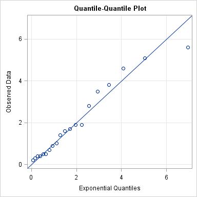
"But, Rick," you might argue, "the plotted points fall neatly along the diagonal line only because you somehow knew to use a scale parameter of 2 in Step 3. What if I don't know what parameter to use?!"

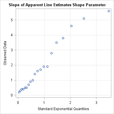
Ahh, but that is the beauty of the Q-Q plot! If you plot the data against the standardized distribution (that is, use a unit scale parameter), then the slope of the line in a Q-Q plot is an estimate of the unknown scale parameter for your data! For example, modify the previous SAS/IML statements so that the quantiles of the exponential distribution are computed as follows: q = quantile("Exponential", v); /* 3 */

The resulting Q-Q plot shows points that lie along a line with slope 2, which implies that the distribution of the data is approximately exponentially distributed with a shape parameter close to 2.

Choice of quantiles for the theoretical distribution

The Wikipedia article on Q-Q plots states, "The choice of quantiles from a theoretical distribution has occasioned much discussion." Wow, is that an understatement! Literally dozens of papers have been written on this topic. SAS uses a formula suggested by Blom (1958): (i - 3/8) / (n + 1/4), i=1,2,...,n. Another popular choice is (i-0.5)/n, or even i/(n+1). For large n, the choices are practically equivalent. See O. Thas (2010), Comparing Distributions, p. 57–59 for a discussion of various choices. In PROC UNIVARIATE, the QQPLOT statement supports the RANKADJ= and NADJ= options to accomodate different offsets for the nummerator and denominator in the formula.

Repeating the construction by using the DATA step

These computations are simple enough to perform by using the DATA step and PROC SORT. For completeness, here is the SAS code:

data A;
input y @@;
datalines;
1.7 1.0 0.5 3.5 1.9 0.7 0.4 
5.1 0.2 5.6 4.6 2.8 3.8 1.4 
1.6 0.9 0.3 0.4 1.9 0.5
;
 
proc sort data=A; by y; run; /* 1 */
data Exp;
set A nobs=nobs;
v = (_N_ - 0.375) / (nobs + 0.25); /* 2 */
q = quantile("Exponential", v, 2); /* 3 */
run;
 
proc sgplot data=Exp noautolegend; /* 4 */
scatter x=q y=y;
lineparm x=0 y=0 slope=1; /* SAS 9.3 statement */
xaxis label="Exponential Quantiles" grid; 
yaxis label="Observed Data" grid;
run;

Use PROC RANK to generate normal quantiles

For the special case of a normal Q-Q plot, you can use PROC RANK to generate the normal quantiles. The Blom transformation of the data is accomplished by using the NORMAL=BLOM option, as described in this SAS Usage note on creating a Q-Q plot.

Use PROC UNIVARIATE for Simple Q-Q Plots

Of course, for this example, I don't need to do any computations at all, since PROC UNIVARIATE supports the exponential distribution and other common distributions. The following statements compute goodness-of-fit tests, overlay a curve on the histogram, and display a Q-Q plot:

proc univariate data=A;
var y;
histogram y / exp(sigma=2); 
QQplot y / exp(theta=0 sigma=2);
run;

However, if you think your data are distributed according to some distribution that is not built into PROC UNIVARIATE, the techniques in this article show how to construct a Q-Q plot to help you assess whether some "named" distribution might model your data.