A popular use of SAS/IML software is to optimize functions of several variables. One statistical application of optimization is estimating parameters that optimize the maximum likelihood function. This post gives a simple example for maximum likelihood estimation (MLE): fitting a parametric density estimate to data.
Which density curve fits the data?
If you plot a histogram for the SepalWidth variable in the famous Fisher's iris data, the data look normally distributed. The normal distribution has two parameters: μ is the mean and σ is the standard deviation. For each possible choice of (μ, σ), you can ask the question, "If the true population is N(μ, σ), how likely is it that I would get the SepalWidth sample?" Maximum likelihood estimation is a technique that enables you to estimate the "most likely" parameters. This is commonly referred to as fitting a parametric density estimate to data.
Visually, you can think of overlaying a bunch of normal curves on the histogram and choosing the parameters for the best-fitting curve. For example, the following graph shows four normal curves overlaid on the histogram of the SepalWidth variable:
proc sgplot data=Sashelp.Iris; histogram SepalWidth; density SepalWidth / type=normal(mu=35 sigma=5.5); density SepalWidth / type=normal(mu=32.6 sigma=4.2); density SepalWidth / type=normal(mu=30.1 sigma=3.8); density SepalWidth / type=normal(mu=30.5 sigma=4.3); run; |
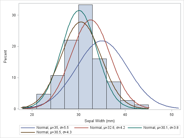
It is clear that the first curve, N(35, 5.5), does not fit the data as well as the other three. The second curve, N(32.6, 4.2), fits a little better, but mu=32.6 seems too large. The remaining curves fit the data better, but it is hard to determine which is the best fit. If I had to guess, I'd choose the brown curve, N(30.5, 4.3), as the best fit among the four.
The method of maximum likelihood provides an algorithm for choosing the best set of parameters: choose the parameters that maximize the likelihood function for the data. Parameters that maximize the log-likelihood also maximize the likelihood function (because the log function is monotone increasing), and it turns out that the log-likelihood is easier to work with. (For the normal distribution, you can explicitly solve the likelihood equations for the normal distribution. This provides an analytical solution against which to check the numerical solution.)
The likelihood and log-likelihood functions
The UNIVARIATE procedure uses maximum likelihood estimation to fit parametric distributions to data. The UNIVARIATE procedure supports fitting about a dozen common distributions, but you can use SAS/IML software to fit any parametric density to data. There are three steps:
- Write a SAS/IML module that computes the log-likelihood function. Optionally, since many numerical optimization techniques use derivative information, you can provide a module for the gradient of the log-likelihood function. If you do not supply a gradient module, SAS/IML software automatically uses finite differences to approximate the derivatives.
- Set up any constraints for the parameters. For example, the scale parameters for many distributions are restricted to be positive values.
- Call one of the SAS/IML nonlinear optimization routines. For this example, I call the NLPNRA subroutine, which uses a Newton-Raphson algorithm to optimize the log-likelihood.
Step 1: Write a module that computes the log-likelihood
A general discussion of log-likelihood functions, including formulas for some common distributions, is available in the documentation for the GENMOD procedure. The following module computes the log-likelihood for the normal distribution:
proc iml;
/* write the log-likelihood function for Normal dist */
start LogLik(param) global (x);
   mu = param[1];
   sigma2 = param[2]##2;
   n = nrow(x);
   c = x - mu;
   f = /* -n/2*log(2*constant('pi')) */ /* Optional: Include this constant value */
       -n/2*log(sigma2) - 1/2/sigma2*sum(c##2);
   return ( f );
finish; |
Notice that the arguments to this module are the two parameters mu and sigma. The data vector (which is constant during the optimization) is specified as the global variable x. When you use an optimization method, SAS/IML software requires that the arguments to the function be the quantities to optimize. Pass in other parameters by using the GLOBAL parameter list.
It's always a good idea to test your module. Remember those four curves that were overlaid on the histogram of the SepalWidth data? Let's evaluate the log-likelihood function at those same parameters. We expect that log-likelihood should be low for parameter values that do not fit the data well, and high for parameter values that do fit the data.
use Sashelp.Iris;
read all var {SepalWidth} into x;
close Sashelp.Iris;

/* optional: test the module */
params = {35   5.5,
          32.6 4.2,
          30.1 3.8,
          30.5 4.3};
LogLik = j(nrow(params),1);
do i = 1 to nrow(params);
   p = params[i,];
   LogLik[i] = LogLik(p);
end;
print Params[c={"Mu" "Sigma"} label=""] LogLik; |
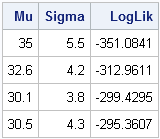
The log-likelihood values confirm our expectations. A normal density curve with parameters (35, 5.5) does not fit the data as well as the other parameters, and the curve with parameters (30.5, 4.3) fits the curve the best because its log-likelihood is largest.
Step 2: Set up constraints
The SAS/IML User's Guide describes how to specify constraints for nonlinear optimization. For this problem, specify a matrix with two rows and k columns, where k is the number of parameters in the problem. For this example, k=2.
- The first row of the matrix specifies the lower bounds on the parameters. Use a missing value (.) if the parameter is not bounded from below.
- The second row of the matrix specifies the upper bounds on the parameters. Use a missing value (.) if the parameter is not bounded from above.
The only constraint on the parameters for the normal distribution is that sigma is positive. Therefore, the following statement specifies the constraint matrix:
/*     mu-sigma constraint matrix */
con = { .   0,  /* lower bounds: -infty < mu; 0 < sigma */
. .}; /* upper bounds: mu < infty; sigma < infty */ |
Step 3: Call an optimization routine
You can now call an optimization routine to find the MLE estimate for the data. You need to provide an initial guess to the optimization routine, and you need to tell it whether you are finding a maximum or a minimum. There are other options that you can specify, such as how much printed output you want.
p = {35 5.5};/* initial guess for solution */
opt = {1,    /* find maximum of function   */
       4};   /* print a LOT of output      */
call nlpnra(rc, result, "LogLik", p, opt, con); |
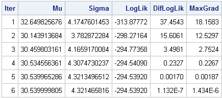
The following table and graph summarize the optimization process. Starting from the initial condition, the Newton-Raphson algorithm takes six steps before it reached a maximum of the log-likelihood function. (The exact numbers might vary in different SAS releases.) At each step of the process, the log-likelihood function increases. The process stops when the log-likelihood stops increasing, or when the gradient of the log-likelihood is zero, which indicates a maximum of the function.
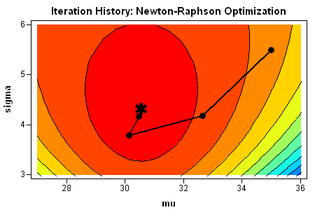
You can summarize the process graphically by plotting the path of the optimization on a contour plot of the log-likelihood function. I used SAS/IML Studio to visualize the path. You can see that the optimization travels "uphill" until it reaches a maximum.
Check the optimization results
As I mentioned earlier, you can explicitly solve for the parameters that maximize the likelihood equations for the normal distribution. The optimal value of the mu parameter is the sample mean of the data. The optimal value of the sigma parameter is the unadjusted standard deviation of the sample. The following statements compute these quantities for the SepalWidth data:
OptMu = x[:]; OptSigma = sqrt( ssq(x-OptMu)/nrow(x) ); |
The values found by the NLPNRA subroutine agree with these exact values through seven decimal places.

38 Comments
Attached are two very compact ways to do this using PROC OPTMODEL in SAS/OR. Note that both LogLikelihood and LogLikelihood2 differ from your LogLik by an additive constant but of course yield the same optimal parameters. Download the OPTMODEL program.
Hi Rob, The code you provided was very helpful for me. I used it with my data and it worked perfect. I am now trying to do the same thing but for Poisson model instead of Normal. I wrote the following code but I am not sure whether it is correct. what's the best way to validate my code? I also need to estimate the parameters of the Lognormal model; do you have any code that would help me do so?
proc optmodel;
set OBS;
num x {OBS};
read data sashelp.iris into OBS=[_N_] x= SepalWidth;
num n = card(OBS);
var lambda>=0 init 0;
max LogLikelihood = sum {i in OBS}(x[i] * log(lambda)) - n * lambda;
/*max LogLikelihood1 = sum {i in OBS}(x[i] * log(lambda)) - log(x[i]) * lambda;
max LogLikelihood2 = sum {i in OBS} log(PDF('poisson',x[i],lambda));
LogLikelihood1 and LogLikelihood2 didn't work*/
solve ;
print lambda;
print LogLikelihood;
num optlambda = (sum {i in OBS} x[i]) / n;
print optlambda;
quit;
Pingback: The “power” of finite mixture models - The DO Loop
Pingback: Modeling the distribution of data? Create a Q-Q plot - The DO Loop
Hi Dr. Rick Wicklin, after running the MLE following above code, if I want to make a data table with the parameters (MU, SIGMA) estimated, how can I do? Thank you very much. Regards, Yong
When you say "make a data table," do you mean display it, or create a SAS data set? To print the results, say
print result;
To create a SAS data set, see http://blogs.sas.com/content/iml/2011/04/18/writing-data-from-a-matrix-to-a-sas-data-set/
Hi Rick Wicklin, pls I have an issue which I will like you help me out on my research.
Actually, I'm working on Polynomial regression, with a particular data, two methods have been used which are Numerical and OLS method with little difference in their results.. Now, I'm trying to contribute using MLE for the same Data.
How can I go abt that on SAS ?
I need a SAS code for this pls help me....
I must present this work some days left...
Many standard models are solvable using PROC GENMOD, which computes MLE. For more sophisticated models, PROC NLMIXED is the SAS procedure that solves general MLE. You can post details of your question, along with sample data, at the SAS Support Communities.
Pingback: Understanding local and global variables in the SAS/IML language - The DO Loop
Dr. Rick Wicklin.. When I have a likelihood function where I have to estimate 3 parameters mu,sigma and Pc (proabability) , can I use the same code ?
For example :likelihood = Pc ∫ f (x) dx where f is a normal distribution with unknown mu and sigma
Also, Can the CDF function be used in the function f that you have defined.
Yes, you should be able to use similar code. Yes, you can call the CDF function from within the likelihood function.
Hi Rick
I am trying to create a vector in which each value is the result of an optimization relevant to the row. To be clearer:
First, I have a column vector called n, composed of the numbers 50 to 40000 in increments of 1
Second, I have a vector P defining the objective function, which is composed of two inputs: known n and unknown S where S needs to be optimized to maximize each row value of P. P is defined by:
P = 50*(S##.45)#(n##1.1)-40000*n-S*n-S##1.35#n##.5
Therefore, I need one optimized value in the S vector per row value of n.
I have tried creating a do-loop in IML but as you know modules cannot be made to start on loops.
I have tried to create a macro but had issues.
Any suggestions on the best way forward?
Yes, post your question, sample data, and code to the SAS/IML Support Community.
PS I did manage to get it right outside of IML. However, this macro do-loop with Proc NLP takes a seriously long time once I loop between 50 and 40000, and I had to disable the log which kept on filling up. Still wondering if there's an easier way in IML :-)
options nonotes nosource nosource2 errors=0;
Data Estimates;
Input S 12.5;
Datalines;
9999.99999
;
Run;
%Macro simul;
%do i = 50 %to 90;
Proc NLP noprint outest=Parms(where=(_TYPE_='PARMS'));
Max P0;
Decvar S;
P0 = 50*(S**.45)*(&i**1.1)-40000-(S*&i)-(S**1.35)*(&i**.5);
Run;
Data Estimates;
Set Estimates Parms(keep=S);
Run;
%end;
%mend;
%simul;
This is a rational expression in the variable S. Use calculus. Take the derivative w/r/t S and set it equal to zero. Solve for the root numerically by using the FROOT function.
What do you mean "modules cannot be made to start on loops." I am not familiar with any restrictions on calling modules within loops or with looping inside a module.
Pingback: Optimizing a function that evaluates an integral - The DO Loop
Hi~~~
This blog's posts are really helpful to my job, thank you^^
I'm working on an statistical MLE job using IML's call NLPQN module. The situation is that initial values are very critical to the stability of the solution and I need to make a simulation with different initial values of more than 100 times. I have looked through the helpdoc or manuals for the way how to store or extract objective function values printed on log window by setting option vector, and however failed to find out _._. The simulation took a long time for the completetion, so I could not watch the objective function value printed in log window in each time of simulation path.
So, I need to get the objective function value at the MLE solution point and store it in a "data set" and use it later, for example, the selection among the simulation results.
If possible, then hessian matrix can be stored in a daa set?
Thank you in advance
I suggest that you post your question and sample data to the SAS/IML Support Community
Hi Rick, can you please share some real world problems where MLE is used?Is it only used to measure the value of mean and sigma of the dataset of the closest fit bell curve? What happens if the data is the dependent variable is driven by multiple factors?
MLE is explained in the Wikipedia article that I linked to in the 2nd paragraph. It is a general method of choosing parameters in a model, including regression models.
Hi again. Can you do this for uniform distribution too between 0 and 1? I don't understand how to incorporate the theta aspect.
Thanks
Yes, you can do it. You can ask statistical and programming questions at the SAS Support Communities.
Hi dr. Rick Wicklin, i've read this article and I saw that you have used the iteration history (of the call nlprna) for the last graph. My question is trivial: how can i save the iteration history of the call nlprna in dataset and what is the procedure who you have used for the last graph? tnx.
Good question. I use ODS OUTPUT to save the iteration history and then used the ContourPlot in IMLPlus to visualize the path. I have added a link in the article to download the program. If you prefer regular SAS, make a similar image by using a GTL template.
Hi Mr Rick Wicklin,
I am studying my statistics thesis about max Extreme Value distribution.
I try to estimate parameters of I. type (Gumbell) distribution via Maximum Likelihood Method on SAS. Is it possible to apply this on SAS ? If yes, could you please share with me related codes ?
Thanks!
Yes, use the UNIVARIATE procedure. The HISTOGRAM statement supports the GUMBEL distribution.
Pingback: Ten tips before you run an optimization - The DO Loop
Pingback: Two ways to compute maximum likelihood estimates in SAS - The DO Loop
If I simulate data for 1000 times from Weibull (a,b) distribution with a is shape parameter and b is scale parameter for different combination od parameters to calculate maximum likelihood estimates (MLEs) for a and b. How the initial values for a and b that needed to calculate MLEs can be specified. For example, If I generate from Weibull(24, 4) and Weibull(12,4) to calculate MLEs, what are the suitable initials for both parameters in the two simulations?
Thank you.
In general, that is a difficult task. Most people just make a guess, such as (1,1). If that guess doesn't converge, then you can try a more sophisticated guess, such as using the method of moments to estimate the parameters that produce the sample mean and variance. See also the article "How to find an initial guess for an optimization."
Hi Rick,
I have a problem choosing initial values for my simulation. I have a bivariate density with 3 parameters but I don't know how to see the graphs so I can make judgement. I followed your blog regarding the evaluation of the loglikelihood which is pretty good and very helpful. But graphing the log-likelihhood may give me a prouder image.
my code is below
Thank you,
Amal
[ long SAS/IML program removed ]
Please post your question and SAS code to the SAS Support Community for SAS/IML programming. For this question, you might want to read
"How to find an initial guess for an optimization" and
"The method of moments: A smart way to choose initial parameters for MLE."
Hi, how do I do a MLE for truncated normal?
I have set up the log-likelihood of the one-sided truncated normal. But I keep getting
ERROR: Invalid Operation.
ERROR: Termination due to Floating Point Exception
data ln;
input dor 8.;
qt=quantile("normal", dor, 0, 1);
datalines;
0.10
0.20
0.15
0.22
0.15
0.10
0.08
0.09
0.12
;
run;
/* obtain number accounts */
%let dsn = ln;
%let dsnid = %sysfunc(open(&dsn));
%let nobs=%sysfunc(attrn(&dsnid,nlobs));
%let rc =%sysfunc(close(&dsnid));
proc sql noprint;
select count(*), mean(qt), std(qt) into :nobs, :mean, :std
from ln;
quit;
%put &nobs.;
%put &mean.;
%put &std.;
proc nlmixed data=LN;
parms mu &mean. sigma &std.; * initial values of parameters;
bounds 0 < sigma; * bounds on parameters;
LL = logpdf("normal", qt, mu, sigma) - &nobs.*logcdf("normal",qt, mu, sigma);
model qt ~ general(LL);
run;
Your LL does not look correct. I'm not sure what interval [a,b] you are using for truncation, but the correct pdf is at my article "Implement the truncated normal distribution in SAS." Notice that the CDF depends on a or b, not on the variable qt.
Hi dr. Rick Wicklin, I'm estimating several parameters with proc nlp ,but I get different results every time I run the code and I have no idea whats wrong . here's my code . THANK YOU!!
proc nlp data=PIN;
max logf;
parms alpha delta eb es mu;
bounds alpha>0;
logf = log((1-alpha) * pdf('POISSON',buy, eb) * pdf('POISSON',sell, es) +
alpha * delta * pdf('POISSON',buy, eb) * pdf('POISSON',sell, es+mu) +
alpha * (1-delta) * pdf('POISSON',buy, eb+mu) * pdf('POISSON',sell, es));
run;
Yes, and if you look in the SAS log you will see
NOTE: Initial value of parameter alpha is set randomly to 0.4956929514.
NOTE: Initial value of parameter delta is set randomly to 0.6510622872.
NOTE: Initial value of parameter eb is set randomly to 0.9358643442.
NOTE: Initial value of parameter es is set randomly to 0.9485867317.
NOTE: Initial value of parameter mu is set randomly to 0.3292414291.
If you don't want random values, then set the values on the PARMS statement.
There are other problems with your program. If you have additional questions, you should post to the SAS Optimization/OR Community.
Pingback: Two tips for optimizing a function that has a restricted domain - The DO Loop