Recently I had to compute the trace of a product of square matrices. That is, I had two large nxn matrices, A and B, and I needed to compute the quantity trace(A*B). Furthermore, I was going to compute this quantity thousands of times for various A and B as part of an optimization problem.
I wondered whether it was possible to compute the trace without actually computing the matrix product, which is an O(n3) operation. After all, the trace is just the sum of the diagonal elements, so maybe it is possible to compute the trace of the product without having to compute any of the off-diagonal elements of the product. That would result in an O(n2) operation, which would save considerable computational time.
A Formula for the Trace of a Matrix Product
It you write down the summation for computing the trace of a matrix product, it turns out that the quantity is equivalent to the sum of the elements of an elementwise product. In symbols,
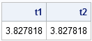
trace(A*B) = sum(A#B`)where '#' denotes elementwise multiplication and B` is the transpose of B. The following example shows SAS/IML statements that compute each quantity:
proc iml; A = rannor( j(5,5) ); /** 5x5 matrix **/ B = rannor( j(5,5) ); /** 5x5 matrix **/ t1 = trace(A*B); t2 = sum(A#B`); print t1 t2; |
A Further Improvement When Either Matrix Is Symmetric
For my application, I could make another computational improvement. The B matrix for my application is symmetric, so that B = B`. In this case, I don't even have to perform the transpose operation for B:
trace(A*B) = sum(A#B) (for symmetric B)
Furthermore, you can use this trick if either of your matrices are symmetric, because it is a general fact that trace(A*B)=trace(B*A) for any square matrices.
Performance Improvement
Computing n2 operations instead of n3 will definitely result in faster execution times, but modern computers are so fast that the improvement is not apparent for small values of n. The following statements time the naive computation and the improved computation for a sequence of matrices of increasing sizes:
/** compute the trace of a product of matrices
    in two different ways **/
size = T(do(100, 1000, 100));
trace = j(nrow(size), 1);
sum = j(nrow(size), 1);

do i = 1 to nrow(size);
   n = size[i];
   x = rannor(j(n,n)); y = rannor(j(n,n));
   t0 = time(); v1 = trace(x*y);
   t1 = time(); v2 = sum(x#y`);
   t2 = time();
   trace[i] = t1 - t0;
   sum[i]   = t2 - t1;
end; |
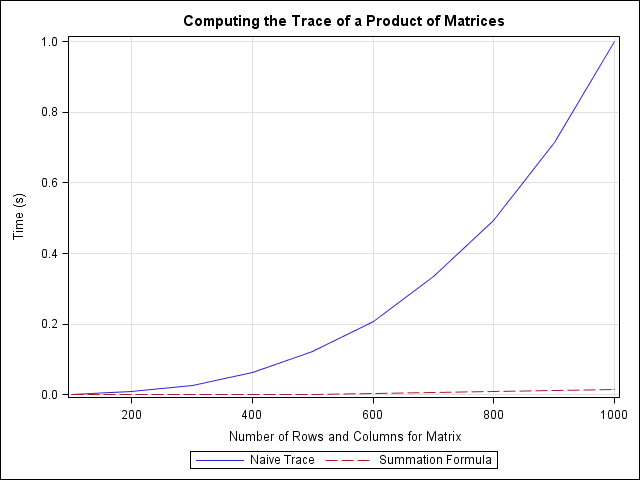
The performance of each method is summarized by the following graph. The blue curve shows the performance of the naive method: computing the trace of the product of matrices by forming the product. This method requires time that increases quickly as the size of the matrices increase. For a 1000 x 1000 matrix, the naive method takes about one second.
In contrast, the red curve shows the performance for computing the sum of the elementwise product. This method is essentially instantaneous for all matrices that were tested. For a 1000 x 1000 matrix, the summation method takes about 0.015 seconds.

3 Comments
Pingback: Computing the diagonal elements of a product of matrices - The DO Loop
But what if you wanted the trace of three matrices?
By associativity, tr(A*B*C) = sum( (A*B)#C` )