Correlation is a fundamental statistical concept that measures the linear association between two variables. There are multiple ways to think about correlation: geometrically, algebraically, with matrices, with vectors, with regression, and more. To paraphrase the great songwriter Paul Simon, there must be 50 ways to view your correlation! But don't "slip out the back, Jack," this article describes only seven of them.

How can we understand these many different interpretations? As the song says, "the answer is easy if you take it logically." These seven ways to view your Pearson correlation are based on the wonderful paper by Rodgers and Nicewander (1988), "Thirteen ways to look at the correlation coefficient," which I recommend for further reading.

1. Graphically

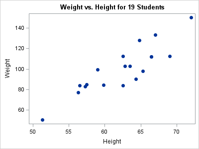
The simplest way to visualize correlation is to create a scatter plot of the two variables. A typical example is shown to the right. (Click to enlarge.) The graph shows the heights and weights of 19 students. The variables have a strong linear "co-relation," which is Galton's original spelling for "correlation." For these data, the Pearson correlation is r = 0.8778, although few people can guess that value by looking only at the graph.

For data that are approximately bivariate normal, the points will align northwest-to-southeast when the correlation is negative and will align southwest-to-northeast when the data are positively correlated. If the point-cloud is an amorphous blob, the correlation is close to zero.

In reality, most data are not well-approximated by a bivariate normal distribution. Furthermore, Anscombe's Quartet provides a famous example of four point-clouds that have exactly the same correlation but very different appearances. (See also the images in the Wikipedia article about correlation.) So although a graphical visualization can give you a rough estimate of a correlation, you need computations for an accurate estimate.

2. The sum of crossproducts

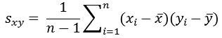
In elementary statistics classes, the Pearson sample correlation coefficient between two variables x and y is usually given as a formula that involves sums. The numerator of the formula is the sum of crossproducts of the centered variables. The denominator involves the sums of squared deviations for each variable. In symbols:

The terms in the numerator involve the first central moments and the terms in the denominator involve the second central moments. Consequently, Pearson's correlation is sometimes called the product-moment correlation.

3. The inner product of standardized vectors

I have a hard time remembering complicated algebraic formulas. Instead, I try to visualize problems geometrically. The way I remember the correlation formula is as the inner (dot) product between two centered and standardized vectors. In vector notation, the centered vectors are x - x̄ and y - ȳ. A vector is standardized by dividing by its length, which in the Euclidean norm is the square root of the sum of the square of the elements. Therefore you can define u = (x - x̄) / || x - x̄ || and v = (y - ȳ) / || y - ȳ ||. Looking back at the equation in the previous section, you can see that the correlation between the vectors x and y is the inner product r = u · v. This formula shows that the correlation coefficient is inavariant under affine transformations of the data.

4. The angle between two vectors

Linear algebra teaches that the inner product of two vectors is related to the angle between the vectors. Specifically, u · v = ||u|| ||v|| cos(θ), where θ is the angle between the vectors u and v. Dividing both sides by the lengths of u and v and using the equations in the previous section, we find that r = cos(θ), where θ is the angle between the vectors.

This equation gives two important facts about the Pearson correlation. First, the correlation is bounded in the interval [-1, 1]. Second, it gives the correlation for three important geometric cases. When x and y have the same direction (θ = 0), then their correlation is +1. When x and y have opposite directions (θ = π), then their correlation is -1. When x and y are orthogonal (θ = π/2), their correlation is 0.

5. The standardized covariance

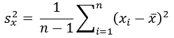
Recall that the covariance between two variables x and y is

The covariance between two variables depends on the scales of measurement, so the covariance is not a useful statistic for comparing the linear association. However, if you divide by the standard deviation of each variable, then the variables become dimensionless. Recall that the standard deviation is the square root of the variance, which for the x variable is given by

Consequently, the expression s_xy / (s_x s_y) is a standardized covariance. If you expand the terms algebraically, the "n - 1" terms cancel and you are left with the Pearson correlation.

6. The slope of the regression line between two standardized variables

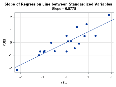
Most textbooks for elementary statistics mention that the correlation coefficient is related to the slope of the regression line that estimates y from x. If b is the slope, then the result is r = b (s_x / s_y). That's a messy formula, but if you standardize the x and y variables, then the standard deviations are unity and the correlation equals the slope.

This fact is demonstrated by using the same height and weight data for 19 students. The graph to the right shows the data for the standardized variables, along with an overlay of the least squares regression line. The slope of the regression line is 0.8778, which is the same as the correlation between the variables.

7. Geometric mean of regression slopes

The previous section showed a relationship between two of the most important concepts in statistics: correlation and regression. Interestingly, the correlation is also related to another fundamental concept, the mean. Specifically, when two variables are positively correlated, the correlation coefficient is equal to the geometric mean of two regression slopes: the slope of y regressed on x (b_x) and the slope of x regressed on y (b_y).

To derive this result, start from the equation in the previous section, which is r = b_x (s_x / s_y). By symmetry, it is also true that r = b_y (s_y / s_x). Consequently, r² = b_x b_y or r = sqrt( b_x b_y ), which is the geometric mean of the two slopes..

Summary

This article shows multiple ways that you can view a correlation coefficient: analytically, geometrically, via linear algebra, and more. The Rodgers and Nicewander (1988) article includes other ideas, some of which are valid only asymptotically or approximately.

If you want to see the computations for these methods applied to real data, you can download a SAS program that produces the computations and graphs in this article.

What is your favorite way to think about the correlation between two variables? Leave a comment.