Maximum likelihood estimation (MLE) is a powerful statistical technique that uses optimization techniques to fit parametric models. The technique finds the parameters that are "most likely" to have produced the observed data. SAS provides many tools for nonlinear optimization, so often the hardest part of maximum likelihood is writing down the log-likelihood function. This article shows two simple ways to construct the log-likelihood function in SAS. For simplicity, this article describes fitting the binomial and lognormal distributions to univariate data.

Always use the log-likelihood function!

Although the method is known as maximum likelihood estimation, in practice you should optimize the log-likelihood function, which is numerically superior to work with. For an introduction to MLE, including the definitions of the likelihood and log-likelihood functions, see the Penn State Online Statistics Course, which is a wonderful reference.

MLE assumes that the observed data x={x₁, x₂, ..., x_n} are independently drawn from some population. You want to find the most likely parameters θ = (θ₁,...,θ_k) such that the data are fit by the probability density function (PDF), f(x; θ). Since the data are independent, the probability of observing the data is the product Π_i f(x_i, θ), which is the likelihood function L(θ | x). If you take the logarithm, the product becomes a sum. The log-likelihood function is
LL(θ | x) = Σ_i log( f(x_i, θ) )

This formula is the key. It says that the log-likelihood function is simply the sum of the log-PDF function evaluated at the data values. Always use this formula. Do not ever compute the likelihood function (the product) and then take the log, because the product is prone to numerical errors, including overflow and underflow.

Two ways to construct the log-likelihood function

There are two simple ways to construct the log-likelihood function in SAS:

• Use the LOGPDF function in SAS. The LOGPDF function supports about 25 common probability distributions.
• Manually apply the LOG function to the PDF formula. Formulas for many popular modeling distributions are included in the "Standard Distributions" section of the PROC MCMC documentation. If the distribution you want is not in that reference, you can use the formula from a textbook, encyclopedia, or journal article.

You can download the SAS program that creates the data and contains all analyses in this article.

Example: The log-likelihood function for the binomial distribution

A coin was tossed 10 times and the number of heads was recorded. This was repeated 20 times to get a sample. A student wants to fit the binomial model X ~ Binom(p, 10) to estimate the probability p of the coin landing on heads. For this problem, the vector of MLE parameters θ is merely the one parameter p.

Recall that if you are using SAS/IML to optimize an objective function, the parameter that you are trying to optimize should be the only argument to the function, and all other parameters should be specified on the GLOBAL statement. Thus one way to write a SAS/IML function for the binomial log-likelihood function is as follows:

proc iml;
/* Method 1: Use LOGPDF. This method works in DATA step as well */
start Binom_LL1(p) global(x, NTrials);
   LL = sum( logpdf("Binomial", x, p, NTrials) );
   return( LL );
finish;
 
/* visualize log-likelihood function, which is a function of p */
NTrials = 10;    /* number of trials (fixed) */
use Binomial; read all var "x"; close;
 
p = do(0.01, 0.99, 0.01);      /* vector of parameter values */
LL = j(1, ncol(p), .);
do i = 1 to ncol(LL);
   LL[i] = Binom_LL1( p[i] );  /* evaluate LL for a sequence of p */
end;
 
title "Graph of Log-Likelihood Function";
title2 "Binomial Distribution, NTrials=10";
call series(p, LL) grid={x y} xvalues=do(0,1,0.1)
                   label={"Probability of Sucess (p)", "Log Likelihood"};

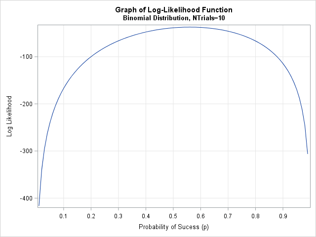
Notice that the data is constant and does not change. The log likelihood is considered to be a function of the parameter p. Therefore you can graph the function for representative values of p, as shown. The graph clearly shows that the log likelihood is maximal near p=0.56, which is the maximum likelihood estimate. The graph is fairly flat near its optimal value, which indicates that the estimate has a wide standard error. A 95% confidence interval for the parameter is also wide. If the sample contained 100 observations instead of only 20, the log-likelihood function might have a narrower peak.

Notice also that the LOGPDF function made this computation very easy. You do not need to worry about the actual formula for the binomial density. All you have to do is sum the log-density at the data values.

In contrast, the second method requires a little more work, but can handle any distribution for which you can compute the density function. If you look up the formula for the binomial PDF in the MCMC documentation, you see that
PDF(x; p, NTrials) = comb(NTrials, x) * p**x * (1-p)**(NTrials-x)
where the COMB function computes the binomial coefficient "NTrials choose x." There are three terms in the PDF that are multiplied together. Therefore when you apply the LOG function, you get the sum of three terms. You can use the LCOMB function in SAS to evaluate the logarithm of the binomial coefficients in an efficient manner, as follows:

/* Method 2: Manually compute log likelihood by using formula */
start Binom_LL2(p) global(x, NTrials);
   LL = sum(lcomb(NTrials, x)) + log(p)*sum(x) + log(1-p)*sum(NTrials-x);
   return( LL );
finish;
 
LL2 = Binom_LL2(p);      /* vectorized function, so no need to loop */

The second formulation has an advantage in a vector language such as SAS/IML because you can write the function so that it can evaluate a vector of values with one call, as shown. It also has the advantage that you can modify the function to eliminate terms that do not depend on the parameter p. For example, if your only goal is maximize the log-likelihood function, you can omit the term sum(lcomb(NTrials, x)) because that term is a constant with respect to p. That reduces the computational burden. Of course, if you omit the term then you are no longer computing the exact binomial log likelihood.

Example: The log-likelihood function for the lognormal distribution

In a similar way, you can use the LOGPDF or the formula for the PDF to define the log-likelihood function for the lognormal distribution. For brevity, I will only show the SAS/IML functions, but you can download the complete SAS program that defines the log-likelihood function and computes the graph.

The following SAS/IML modules show two ways to define the log-likelihood function for the lognormal distribution. For the lognormal distribution, the vector of parameters θ = (μ, σ) contains two parameters.

/* Method 1: use LOGPDF */
start LogNormal_LL1(param) global(x);
   mu = param[1];
   sigma = param[2];
   LL = sum( logpdf("Lognormal", x, mu, sigma) );
   return( LL );
finish;
 
/* Method 2: Manually compute log likelihood by using formula
   PDF(x; p, NTrials) = comb(NTrials,x) # p##x # (1-p)##(NTrials-x)
*/
start LogNormal_LL2(param) global(x);
   mu = param[1];
   sigma = param[2];
   twopi = 2*constant('pi');
   LL = -nrow(x)/2*log(twopi*sigma##2) 
        - sum( (log(x)-mu)##2 )/(2*sigma##2)
        - sum(log(x));  /* this term is constant w/r/t (mu, sigma) */
   return( LL );
finish;

The function that uses the LOGPDF function is simple to write. The second method is more complicated because the lognormal PDF is more complicated than the binomial PDF. Nevertheless, the complete log-likelihood function only requires a few SAS/IML statements.

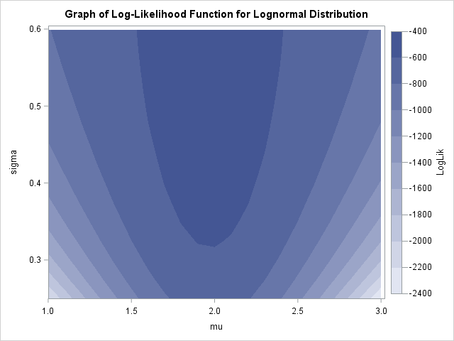
For completeness, the contour plot on this page shows the log-likelihood function for 200 simulated observations from the Lognormal(2, 0.5) distribution. The parameter estimates are (μ, σ) = (1.97, 0.5).

Summary

This article has shown two simple ways to define a log-likelihood function in SAS. You can sum the values of the LOGPDF function evaluated at the observations, or you can manually apply the LOG function to the formula for the PDF function. The log likelihood is regarded as a function of the parameters of the distribution, even though it also depends on the data. For distributions that have one or two parameters, you can graph the log-likelihood function and visually estimate the value of the parameters that maximize the log likelihood.

Of course, SAS enables you to numerically optimize the log-likelihood function, thereby obtaining the maximum likelihood estimates. My next blog post shows two ways to obtain maximum likelihood estimates in SAS.