At SAS Global Forum last week, I saw a poster that used SAS/IML to optimized a quadratic objective function that arises in financial portfolio management (Xia, Eberhardt, and Kastin, 2017). The authors used the Newton-Raphson optimizer (NLPNRA routine) in SAS/IML to optimize a hypothetical portfolio of assets.

The Newton-Raphson algorithm is one of my favorite optimizers. However, for a quadratic objective function there is a simpler choice. You can use the NLPQUA function in SAS/IML to optimize a quadratic objective function.

Optimize an unconstrainted quadratic objective function in SAS/IML

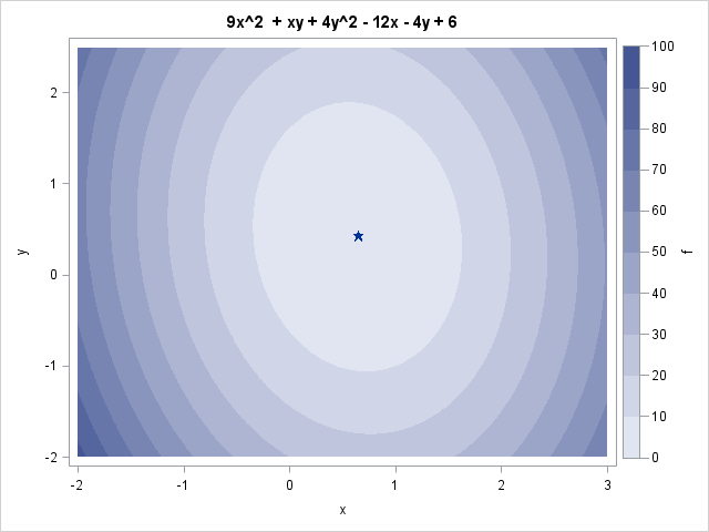
Let's see how this works by specifying a quadratic polynomial in two variables. The function is
f(x,y) = (9*x##2 + x#y + 4*y##2) - 12*x - 4*y + 6
       = 0.5*x` H x + L x + 6
where H = {18  1, 1  8} is a 2x2 symmetric matrix, L = {-12  -4} is a row vector, and x = {x, y} is a column vector.

To use the NLPQUA subroutine, you need to write down the Hessian matrix, H, which is the symmetric matrix of second derivatives. Of course, for a quadratic function the second derivatives are constants. In the following SAS/IML program, the matrix H contains the second derivatives and the vector lin contains the coefficients for the linear and constant terms of f:

/* objective function is
   f(x,y) = (3*x-2)##2 + (2*y-1)##2 + x#y + 1
          = (9*x##2  + x#y + 4*y##2)  + -12*x  - 4*y + 6
   grad(f) = g(x,y) = [ 18*x + y - 12,  x + 8*y - 4 ]
   hess(f)  = [ dg1/dx  dg2/dx ]  =  [ 18  1 ]
              [ dg1/dy  dg2/dy ]     [  1  8 ]
*/
proc iml;
H = {18 1,             /* matrix of second derivatives */
      1 8};
lin = { -12 -4 6 };    /* vector of linear terms and the constant term */

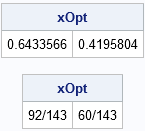
The NLPQUA subroutine enables you to specify the Hessian matrix and the linear coefficients. From those values, the routine uses an efficient solver to find the global minimum of the quadratic polynomial, which occurs at x=92/143, y=60/143:

x0 = j(1, 2, 1);       /* initial guess */
opt = {0 1};           /* minimize, print final parameters */
call nlpqua(rc, xOpt, H, x0, opt) lin=lin;
print xOpt; 
print xOpt[format=Fract.];

Solve a constrained quadratic program in SAS/IML

You can also use the NLPQUA subroutine to solve a constrained problem. Suppose that you are only interested in values of (x,y) in the unit square and you require that the solution satisfies the linear constraint x + y = 1. In that case you can define a matrix that specifies the linear constraints as follows:

blc = {0 0 . .,   /* lower bound: 0 <= x_i        */
       1 1 . .,   /* upper bound:      x_i <= 1   */
       1 1 0 1};  /* linear constraint x +  y = 1 */
call nlpqua(rc, conOpt, H, x0, opt, blc) lin=lin;
print conOpt[format=Fract.];

Notice how the linear constraints are specified for this (and every other) NLP function. Let p be the number of parameters in the problem. The first p elements of the first row specify the lower bounds for the parameters; use a missing value for variables that are not bounded below. The last two columns of the first row are not used, so you should always set those elements to missing values. Similarly, the first p elements of the second row specify the upper bound for the variables. The last two columns of the second row are not used, so set those elements to missing values.

Additional rows specify coefficients for the linear constraint. An equality constraint of the form a₁*x₁ + a₂*x₂ + ... + a_n *x_n = c is encoded as a row of coefficients {a₁ a₂ ... a_n 0 c}, where the 0 in the penultimate location indicates equality. A "less than" inequality of the form a₁*x₁ + a₂*x₂ + ... + a_n *x_n ≤ c is encoded as the row {a₁ a₂ ... a_n  -1  c}, where the -1 indicates the "less than or equal" symbol. Similarly, a value of +1 in the penultimate location indicates the "greater than or equal" symbol (≥). See the documentation for the NLP routines for additional details about specifying constraints.

Solve quadratic programs in PROC OPTMODEL

If you have access to SAS/OR software, PROC OPTMODEL provides a simple and natural language for solving simple and complex optimization problems. For this problem, PROC OPTMODEL detects that the objective function is quadratic and automatically chooses an efficient QP solver. Here is one way to solve the unconstrained and constrained problems in PROC OPTMODEL. The answers are the same as before and are not shown.

/* variable names x and y */
proc optmodel;
   /* unconstrained quadratic optimization */
   var x, y;
   min f = 9*x^2 + x*y + 4*y^2 - 12*x - 4*y + 6;
   solve;                    /* call QP solver */
   print x Fract. y Fract.;
 
   /* constrained quadratic optimization */
   x.lb = 0; x.ub = 1;        /* bounds on variables */
   y.lb = 0; y.ub = 1;
   con SumToOne:              /* linear constraint */
      x + y = 1;
   solve;                     /* call QP solver */
   print x Fract. y Fract.;
quit;

In summary, if you want to optimize a quadratic objective function (with or without constraints), use the NLPQUA subroutine in SAS/IML, which is a fast and efficient way to maximize or minimize a quadratic function of many variables. If you have access to SAS/OR software, PROC OPTMODEL provides an even simpler syntax.