Many univariate descriptive statistics are intuitive. However, weighted statistic are less intuitive. A weight variable changes the computation of a statistic by giving more weight to some observations than to others. This article shows how to compute and visualize weighted percentiles, also known as a weighted quantiles, as computed by PROC MEANS and PROC UNIVARIATE in SAS. Recall that percentiles and quantiles are the same thing: the 100p^th percentile is equal to the p^th quantile.

I do not discuss survey data in this article. Survey statisticians use weights to make valid inferences in survey data, and you can see the SAS documentation to learn about how to use weights to estimate variance in complex survey designs.

Weights vs frequencies

Before we calculate a weighted statistic, let's remember that a weight variable is not that same as a frequency variable. A frequency variable, which associates a positive integer with each observation, specifies that each observation is replicated a certain number of times. There is nothing unintuitive about the statistics that arise from including a frequency variable. They are the same that you would obtain by duplicating each record according to the value of the frequency variable.

Weights are not frequencies. Weights can be fractional values. When comparing a weighted and unweighted analyses, the key idea is this: an unweighted analysis is equivalent to a weighted analysis for which the weights are all 1. An "unweighted analysis" is really a misnomer; it should be called an "equally weighted" analysis!

Unweighted percentiles

To understand how weights change the computation of percentiles, let's review the standard unweighted computation of the empirical percentiles (or quantiles) of a set of n numbers. First, sort the data values from smallest to largest. Then construct the empirical cumulative distribution function (ECDF). Recall that the ECDF is a piecewise-constant step function that increases by 1/n at each data point. The quantity 1/n represents the fact that each observation is weighted equally in this analysis.

The quantile function is derived from the CDF function, and the quantile function for a discrete distribution is also a step function. You can use the graph of the ECDF to compute the quantiles. For example, suppose your data are
    { 1    1.9    2.2    3    3.7    4.1    5 }
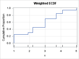
The following graph shows the ECDF for these seven values:

The data values are indicated by tick marks along the horizontal axis. Notice that the ECDF jumps by 1/7 at each data value because there are seven unique values.

I should really show you the graph of the quantile function (an "inverse function" to the CDF), but you can visualize the graph of the quantile function if you rotate your head clockwise by 90 degrees. To find a quantile, start at some value on the Y axis, move across until you hit a vertical line, and then drop down to the X axis to find the datum value. For example, to find the 0.2 quantile (=20th percentile), start at Y=0.2 and move right horizontally until you hit the vertical line over the datum 1.9. Thus 1.9 is the 20th percentile. Similarly, the 0.6 quantile is the data value 3.7. (I omit details about what to do if you hit a horizontal line.)

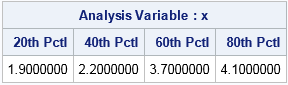
Of course, SAS can speed up this process. The following call to PROC MEANS displays the 20th, 40th, 60th, and 80th percentiles:

data A;
input x wt;
datalines;
1    0.25
1.9  0.05
2.2  0.15
3.0  0.25
3.7  0.15
4.1  0.10
5    0.05
;
 
proc means data=A p20 p40 p60 p80;
   var x;                         /* unweighted analysis: data only */
run;

Weighted percentiles

The previous section shows the relationship between percentile values and the graph of the ECDF. This section describes how the ECDF changes if you specify unequal weights for the data. The change is that the weighted ECDF will jump by the (standardized) weight at each data value. Because the weights sum to unity, the CDF is still a step function that rises from 0 to 1, but now the steps are not uniform in height. Instead, data that have relatively large weights produce a large step in the graph of the ECDF function.

In the previous section, the DATA step defined a weight variable. The weights for this example are
    { 0.25    0.05    0.15    0.25    0.15    0.10    0.05 }
The following graph shows the weighted ECDF for these weights:

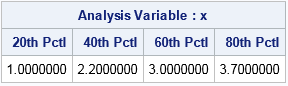
By using this weighted ECDF, you can read off the weighted quantiles. For example, to find the 0.2 weighted quantile, start at Y=0.2 and move horizontally until you hit a vertical line, which is over the datum 1.0. Thus 1.0 is the 20th weighted percentile. Similarly, the 0.6 quantile is the data value 3.0. You can confirm this by calling PROC MEANS with a WEIGHT statement, as shown below:

proc means data=A p20 p40 p60 p80;
   weight wt;                      /* weighted analysis */
   var x;
run;

An intuitive visualization of weighted percentiles

You can use a physical model to intuitively understand weighted percentiles. The model is the same as I used to visualize a weighted mean. Namely, imagine a point-mass of w_i concentrated at position x_i along a massless rod. Finding a weighted percentile p is equivalent to finding the first location along the rod (moving from left to right) at which the proportion of the weight is greater than p. (I omit how to handle special percentiles for which the proportion is equal to p.)

The physical model looks like the following:

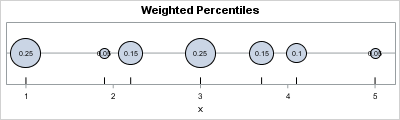
From the figure you can see that x₁ is the p^th quantile for p < 0.25. Similarly, x₂ is the p^th quantile for 0.25 < p < 0.30, and so forth.

If you want to apply these concepts to your own data, you can download the SAS program that generates the CDF graphs and computes the weighted percentiles.

A weighted box plot in SAS

A box plot is composed of quantiles, so you can make a weighted box plot by using weighted quantiles. The following example use PROC SGPLOT (SAS 9.4M1 or later) to create a weighted box plot from the MPG_City variable in the Sashelp.Cars data. The weight (in pounds) of each vehicle is used as the WEIGHT variable. You can compare the location of the boxes and whiskers to the weighted quantiles that you get by using PROC UNIVARIATE and the VARDEF=WEIGHT option.

title "Weighted Box Plot";
proc sgplot data=sashelp.cars;
   vbox mpg_city / weight=weight displaystats=(Mean Q3 Median Q1);
   yaxis grid;
run;
 
proc univariate data=sashelp.cars vardef=weight;
   var mpg_city;
   weight weight;
run;

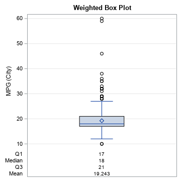
The output from PROC UNIVARIATE is not shown, but the values of the weighted quantiles match the values in the weighted box plot.