I recently read an argument by Andrew Wheeler for using a logarithmic axis for plotting odds ratios. I found his argument convincing. Accordingly, this blog post shows how to create an odds ratio plot in SAS where the ratio axis is displayed on a log scale. Thanks to Bob Derr who read and commented on an early draft of this article.

As the name implies, the odds ratio is a ratio of two odds. You can look up a detailed explanation, but essentially it is the odds of an event occurring in one group divided by the odds of it occurring in another group. The odds ratio is always positive, and an odds ratio of 1 means that the odds of the event occurring in the two groups is the same.

When plotting an odds ratio, the relevant fact is that it is a ratio. A ratio is not symmetric, and reversing the comparison group results in the reciprocal of the ratio. For example, suppose the odds ratio of a disease is 10 when comparing females to males. This means that the odds of getting the disease for females is 10 times greater than for males. However, it is just as correct to say that the odds ratio is 0.1 when you reverse the groups and compare males to females.

On a linear scale, the distance between 0.1 and 1 appears much smaller than the distance between 1 and 10. However, on a log scale, the distance between 10^-1 and 10⁰ (=1) is the same as the distance between 1 and 10¹; on a log₁₀ scale, both distances are 1. It is only by using a log scale that you can visually compare the magnitudes of confidence intervals and standard errors in an odds ratio plot.

The following example is from a SAS Note about estimating odds ratios. In the following example, patients with one of two diagnoses (complicated or uncomplicated) are treated with one of three treatments (A, B, or C) and the result (cured or not cured) is observed:

data uti;
   input diagnosis : $13. treatment $ response $ count @@;
   datalines;
complicated    A  cured 78  complicated   A not 28
complicated    B  cured 101 complicated   B not 11
complicated    C  cured 68  complicated   C not 46
uncomplicated  A  cured 40  uncomplicated A not 5
uncomplicated  B  cured 54  uncomplicated B not 5
uncomplicated  C  cured 34  uncomplicated C not 6
;
proc logistic data=uti plots(only)=oddsratio;
   freq count;
   class diagnosis treatment / param=glm;
   model response(event="cured") = diagnosis treatment diagnosis*treatment ;
   oddsratio treatment;
   oddsratio diagnosis;
   ods output OddsRatiosWald= ORPlot;  /* save data for later use */
run;

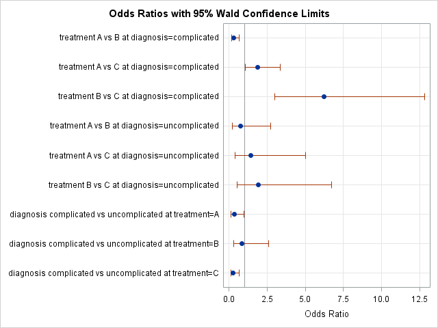
The default odds ratio plot is shown. Five estimates are less than 1 and four are greater than 1. Four confidence intervals intersect 1, which indicates ratios that are not significantly different from 1.

These intervals are not adjusted for multiple comparisons, so you really shouldn't compare their lengths, but many people use the length of a confidence interval to visualize uncertainty in an estimate, and comparisons are inevitable. From looking at the graph, a casual reader might think that the uncertainty for the third ratio (treatment B vs C at diagnosis=complicated) is the biggest. However, this initial impression ignores the fact that the confidence intervals squished into the interval (0,1] might span several orders of magnitude!

Plotting the odds ratios on a log scale automatically

Several SAS procedures enable you to specify a log scale by using the procedure syntax. For example, the LOGISTIC, GLIMMIX, and FREQ procedures support the LOGBASE=10 option on the PLOTS=ODDSRATIO option to generate the plot automatically, as follows:

proc logistic plots=oddsratio(logbase=10); /* specify log scale */
...
run;

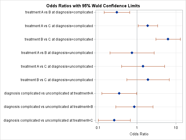
The new odds ratio plot (click to enlarge) displays exactly the same data, but uses a log scale. In the second graph you can see that the confidence interval for the third item is no longer the widest. This plot presents a more faithful visual description of the uncertainty associated with each estimate, regardless of whether the estimate is less than 1 or greater than 1.

Even comparing estimates is much improved. In the first plot, the sixth ratio (treatment B vs C at diagnosis=uncomplicated), which has the value 1.9, seems to be the second most extreme estimate. In the second plot, you can also see that the first and last estimates are more extreme (further from 1) than the sixth estimate. For example, the last estimate is about 0.26, which is the equivalent to the inverse ratio 1/0.26 ≈ 3.8, which is much greater than 1.9. That fact was not evident in the first plot.

Plotting the odds ratios on a log scale manually

If you compute the odds ratio and confidence limits in a DATA step or in a procedure that does not support odds ratio plots, you can use the SGPLOT procedure to create the odds ratio plot with a logarithmic axis. You can use the SCATTER statement to plot the estimates and the XERRORLOWER= and XERRORUPPER= options to plot the confidence intervals. You can use the TYPE=LOG option on the XAXIS statement to change the scale of the axis. The following PROC SGPLOT statement plots the data in the ORPlot data set, which was created by the ODS OUTPUT statement during the first call to PROC LOGISTIC. The names of the data set variables are self-explanatory:

title "Odds Ratios with 95% Wald Confidence Limits";
proc sgplot data=ORPlot noautolegend;
   scatter y=Effect x=OddsRatioEst / xerrorlower=LowerCL xerrorupper=UpperCL
           markerattrs=(symbol=diamondfilled);
   refline 1 / axis=x;
   xaxis grid type=log label="Odds Ratio (log scale)";  /* specify log scale */
   yaxis grid display=(nolabel) discreteorder=data reverse;
run;

The graph is essentially the same as the one produced by PROC LOGISTIC and is not shown. This same technique can be used to create forest plots in SAS.

Create an odds ratio plot with a log scale? You decide!

Should you use a log-scale axis for an odds ratio plot? It depends on your target audience. I recommend it when you are presenting results to a mathematically sophisticated audience.

For other audiences, it is less clear whether the advantages of a log scale outweigh the disadvantages. Odds ratio plots are used heavily in medical research, such as to report the results of clinical trials. Is the average medical practitioner and healthcare administrator comfortable enough with log scales to justify using them?

What do you think? If you use odds ratio plots in your work, which version do you prefer? SAS software can easily produce both kinds of odds ratio plots, so the choice is yours.