Last week's post about odds ratio plots in SAS made me think about a similar plot that visualizes the parameter estimates for a regression analysis. The so-called regression coefficient plot is a scatter plot of the estimates for each effect in the model, with lines that indicate the width of 95% confidence interval (or sometimes standard errors) for the parameters. A sample regression coefficient plot is shown. Variables whose confidence intervals intersect the reference line at 0 are not significant. This article describes how to construct coefficient plots in SAS.

In contrast to the odds ratio plot, SAS procedures do not produce a coefficient automatically, but almost every SAS procedure has an option to produce a parameter estimates table that contains estimates, standard errors, and confidence intervals. By using the ODS OUPUT statement and PROC SGPLOT, it is easy to turn this table into a regression coefficient plot.

A coefficient plot of continuous regressors

The simplest example is for ordinary least squares (OLS) regression on continuous variables. The following data is presented in the documentation for PROC REG. The data specifies "the percentage of raw material that responds in a reaction" according to five explanatory variables. The PROC REG statement runs a main-effects model and uses the CLB option on the MODEL statement to request confidence limits for the coefficients. The ODS OUTPUT statement writes the ParameterEstimates table to a SAS data set called ParamEst.

%let XVars = FeedRate Catalyst AgitRate Temperature Concentration;
data reaction;
input &XVars ReactionPercentage @@;
datalines;
10.0   1.0  100   140  6.0   37.5  10.0   1.0  120   180  3.0   28.5
10.0   2.0  100   180  3.0   40.4  10.0   2.0  120   140  6.0   48.2
15.0   1.0  100   180  6.0   50.7  15.0   1.0  120   140  3.0   28.9
15.0   2.0  100   140  3.0   43.5  15.0   2.0  120   180  6.0   64.5
12.5   1.5  110   160  4.5   39.0  12.5   1.5  110   160  4.5   40.3
12.5   1.5  110   160  4.5   38.7  12.5   1.5  110   160  4.5   39.7
;
ods graphics off;
proc reg data=reaction;
   model  ReactionPercentage = &XVars / CLB;
   ods output ParameterEstimates = ParamEst;
quit;

The data set contains four variables that are need to create the coefficient plot. The Variable variable contains the name of the effects, the Estimate variable contains the parameter estimates, and the LowerCL and UpperCL variables contain the lower and upper limits, respectively, for the 95% confidence interval for the parameters. The following call to the SGPLOT procedure arranges each parameter on the Y axis in the order in which they are specified in the model. The estimates and confidence intervals are plotted on the X axis for each parameter. (An alternative ordering, which I recommend, is to sort the ParamEst data by the size of the estimate before you create the graph.)

/* OPTIONAL SORT: proc sort data=ParamEst;  by Estimate;  run; */
title "Parameter Estimates with 95% Confidence Limits";
proc sgplot data=ParamEst noautolegend;
   scatter y=Variable x=Estimate / xerrorlower=LowerCL xerrorupper=UpperCL
           markerattrs=(symbol=diamondfilled);
   refline 0 / axis=x;
   xaxis grid;
   yaxis grid display=(nolabel) discreteorder=data reverse;
run;

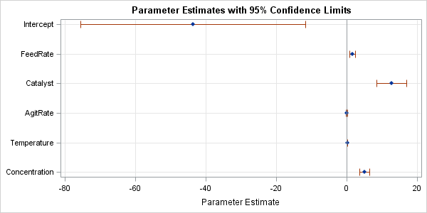
The graph (click to enlarge) is dominated by the large estimate and confidence interval for the Intercept parameter. Consequently, it is difficult to see the range of the confidence intervals for the small parameters. You have to look at the original table of estimates in order to conclude that the AgitRate variable is not significant (the interval contains 0) whereas the Temperature variable is highly significant.

This example demonstrates why these plots are not always useful. In many cases the varied magnitudes of the coefficients result in a coefficient plot that does not visualize the complete set of parameter estimates well. The analyst is forced to look at the table itself to supplement the insights from the coefficient plot.

Incidentally, if you want the half-width of the intervals to be one standard error, you can use a simple DATA step to create the upper and lower limits. For example, Lower = Estimate - StdErr and Upper = Estimate + StdErr.

Coefficient plots for other models

You can also create coefficient plot from the parameter estimates produced by other SAS regression procedures. However, be aware that the names of the variables in the ODS OUTPUT data set might differ from procedure to procedure. There might also be rows in the parameter estimates table that do not correspond to regression effects. For example, the following statements call the ROBUSTREG procedure to compute robust estimates for the same main-effects model:

proc robustreg data=reaction method=M;
   model  ReactionPercentage = &XVars;
   ods output ParameterEstimates = RobParamEst;
quit;

The format of the ParameterEstimates table in the ROBUSTREG procedure is slightly different from the REG version. Whereas REG uses Variable as the name of the column that identifies the parameters, the ROBUSTREG procedure uses Parameter. Consequently, always look at the names of the variables produced by the particular procedure that you are using. The names for the lower and upper confidence limits might also vary across procedures.

The ParameterEstimates table for the robust fit includes a "Scale" parameter, which is fit as part of the model. The parameter estimates from PROC GENMOD also includes a row for a "Scale" parameter.

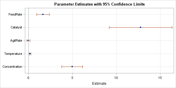
The following call to PROC SGPLOT uses a WHERE clause to omit the estimate of "Scale." I've also excluded the "Intercept" estimate to focus the visualization on the other estimates.

proc sgplot data=RobParamEst noautolegend;
   where Parameter not in ("Intercept" "Scale");
   scatter y=Parameter x=Estimate / xerrorlower=LowerCL xerrorupper=UpperCL
           markerattrs=(symbol=diamondfilled);
   refline 0 / axis=x;
   xaxis grid;
   yaxis grid display=(nolabel) discreteorder=data reverse
         offsetmin = 0.1 offsetmax = 0.1;
run;

The graph is shown at the top of this article. With the intercept estimate gone, you can now resolve the small intervals around the estimates for AgitRate and Temperature.

Using coefficient plots to compare models

One application of the coefficient plot is to provide a visual comparison of different regression models. You can merge the results from different models that use the same explanatory variables but different estimation methods. The following statements merge the results from the OLS and robust regressions:

data All;
set ParamEst(rename=(Variable=Parameter) in=Reg)
    RobParamEst(where=(Parameter^="Scale"));
if Reg then Type="OLS   "; else Type="Robust";
run;
 
proc sgplot data=All;
   where Parameter ^= "Intercept";
   scatter y=Parameter x=Estimate / xerrorlower=LowerCL xerrorupper=UpperCL
           markerattrs=(symbol=diamondfilled)
           group=Type groupdisplay=cluster; /* display side-by-side estimates */
   refline 0 / axis=x;
   xaxis grid min= -1;
   yaxis grid colorbands=odd display=(nolabel) discreteorder=data reverse;
run;

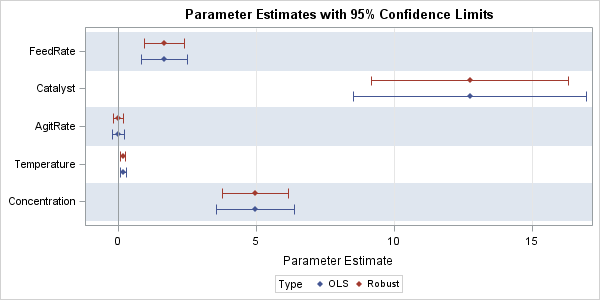
For this plot, the COLORBANDS= option is used to add alternating horizontal stripes to the plot. The estimates are grouped by using the Type variable, and GROUPDISPLAY=CLUSTER option slightly offsets the estimates for each group. The plot makes it apparent that the robust estimates are about the same, but the robust confidence intervals are smaller than the corresponding OLS intervals.

Conclusions

The coefficient plot can be a useful tool for visualizing estimates in a regression model with many parameters. It has difficulties for models that have widely varying parameter estimates. This article show how to use ODS OUPTUT and the SGPLOT procedure to create regression coefficient plots in SAS.

Coefficient plots seems to have found favor with social scientists. The following references provide more details.

• Kastellec and Leoni, 2007, "Using Graphs Instead of Tables in Political Science"
• The coefficient plot is implemented in the coefplot() function in the arm package in R, which accompanies the book Data Analysis Using Regression and Multilevel/Hierarchical Models (Gelman and Hill, 2007).